You already write software. This book helps you use that experience to build, evaluate and run AI
systems. Start with a working baseline and keep asking what your results really support.
Check your starting point
Try these without an assistant writing the first attempt. Documentation is fine. This is a
self-check, not a timed exam.
Read a CSV with Python, count missing values, and write a function with one meaningful test.
Make a Git commit and explain what it includes and excludes.
Call an HTTP endpoint, inspect a failed response, and keep credentials out of commits.
Explain the difference between a percentage and a percentage-point change: from 20% to 25%
is 5 percentage points and a 25% relative increase.
Explain why (100, 1) + (100,) can create an unexpected array. If this is new,
Chapter 2 teaches it.
If the first three are new, start with the programming resources in
Chapter 1. If only the number work is new, begin the normal
path. You can write your first baseline before finishing any mathematics textbook.
Your next useful hour
Create a repository and a learning log. Write one sentence naming a person, a decision and the data
that might help: “A support lead wants to spot tickets that need escalating, using information
available when the ticket arrives.” Then follow
orientation week.
Choose one role to explore while keeping up the shared foundations. The role branches in
Chapter 7 explain what to build, what to explain and what to
recognise. You do not have to finish every branch.
The book has three reading layers
Core. Follow the chapter plan, work through its example, and try the exercise before opening the
answer. Each chapter ends with something you can show.
Practice. Diagnose a failure, compare alternatives, and note the limits of a result. Build on
the same project where the domain and data make sense.
Research. Optional notes and annotated resources go deeper. Treat a recent paper as something to
understand and test, not as a default production choice.
Website reading times cover reading only. Practice-hour figures are planning estimates for
someone who already develops software, not measured completion times.
Two ways to work on the same path
The reference lab gives you synthetic data, reproducible commands, filled-in
reports and deliberate failures. Run it locally with Python. Its results illustrate its stated
assumptions, not real commercial impact.
Your own project uses data you found and are allowed to use. Start with the dataset checklist in
Chapter 2. As soon as you know what you want to predict, set aside a test set, before you look at
the outcomes or fit any preprocessing, and leave it alone until the end. If your data cannot support
the next claim, make the claim smaller or find better data. The reference lab is always there for
practice.
A useful completion standard
Work is finished when you can run it from a clean checkout, explain one decision that mattered,
diagnose a plausible failure, and show a result with its limits. Documentation can stay open. An
honest, reproducible negative or inconclusive comparison is a finished analysis too.
Read offline
The website includes a complete print edition and an EPUB download. Interactive figures also have
static explanations, and the Python lab runs without a model API. Reading progress is saved only in
this browser on this device, and you can clear it from the reader controls.
A working developer's path into AI and machine learning.
The short version. Eight core chapters take you from shipping software to shipping AI systems in
about 450 hours. A ninth applied chapter covers offer recommendation, price recommendation and
churn, with model choices and a full business decision workflow. You build on one thread — one
dataset becomes one model becomes one AI product. Each chapter has a practical plan and a
resources folder for deeper reading.
This is written for someone who already writes software. You use Git, you call APIs, you have
deployed something, and you can read a stack trace without panic. What you want is a clear route
into machine learning and AI engineering, without spending six months on material that turns out to
be out of date.
If you are not yet programming, this book will be hard going. From a standing start, add a
substantial programming stage before these chapter budgets. A planning allowance of 1,000 to
1,500 total hours is an estimate, not a measured completion time or a job guarantee.
CS50P is an excellent place to begin, and this book will still
be here afterwards. You will move through it much faster.
A word on what this can and cannot promise. It is a well-researched, carefully checked path, and I
think it is a good one. It is not the only good one, and it will not fit everyone. Where the
evidence is genuinely mixed, I have tried to say so rather than sound more certain than I am.
How to read this book
Follow the core chapters in order. Chapter 9 is an applied track after Chapters 3 and 6. Use one
guide as your Chapter 7 capstone, or work through all three afterwards. Everything optional is
marked as optional. When you are unsure what to do next, do the next thing on the list. Most
roadmaps offer a branching menu, and that turns out to be part of the problem: a long list of
choices is easy to browse and hard to finish.
Build something in every stage.Dunlosky and colleagues' 2013 review rated practice
testing and distributed practice highly across the learning conditions it examined. Re-reading and
highlighting were less useful overall.
Roediger and Karpicke's 2006 experiments found
that recalling studied text, rather than studying it again, helped people remember it later.
Neither study tests a software curriculum directly. This book applies their ideas: explain from
memory, space out sessions, and build the key exercise with the tutorial closed. Then use your
references to check and correct the result.
Keep a short log. One file, one line per session: the date, the hours, what you built, and what
broke. It gives you a way to revise, and it is a genuinely good answer when someone asks how you
learned all this.
Give yourself room. The plan below assumes ten to twelve hours a week, not twenty. A slower plan
you finish is worth more than a faster one you abandon, and there is no prize for rushing.
Find one place to ask questions. You will get stuck, and a stuck hour with no one to ask is how
most self-study ends. Pick one community early and use it: the
fast.ai forums, the
DataTalks.Club Slack, or the
Hugging Face forums are all free, active and kind to beginners.
Ask with what you tried and what you saw. That habit is itself a skill people hire for.
When you feel lost, do this: open the chapter you are on, find the week plan near the top, and
do only that week's row. Use the resource list to look things up, not to hunt for a better next
hour.
Start here: your first week
If eight chapters and forty-four weeks feel like a lot, start smaller. Week 0 is eight hours.
You do not need to understand machine learning yet. You need a target role, a public repo, a log
file, and a notebook that runs. The day-by-day plan for that week is at the top of
Chapter 1.
End of week 0: you have a public repo, a log, a role, and Colab working. Open
Chapter 2 and follow Week 1 of its plan.
The path at a glance
The diagram shows the order. The table gives each chapter’s time budget and outcome. Start
Chapter 8 alongside Chapter 6 in week 33. Chapter 9 is an
applied extension after Chapters 3 and 6, and can be your Chapter 7 capstone.
flowchart TB
accTitle: The core learning path
accDescr: Complete foundations, machine learning and AI engineering in order, then choose one specialisation. Job search begins alongside production in week 33.
F["Foundations<br/>Ch 1–2 · weeks 0–5"]
M["Machine learning<br/>Ch 3–4 · weeks 6–22"]
E["AI engineering<br/>Ch 5–6 · weeks 23–37"]
S{"Choose one role<br/>Chapter 7"}
A["AI<br/>Engineer"]
B["ML<br/>Engineer"]
C["Data<br/>Scientist"]
F --> M --> E --> S
S --> A
S --> B
S --> C
classDef data fill:#EFF6FF,stroke:#3973AC,color:#17324D,stroke-width:1.5px
classDef model fill:#EFF2FD,stroke:#596FC2,color:#17324D,stroke-width:1.5px
classDef decision fill:#FFF5DF,stroke:#A8751A,color:#17324D,stroke-width:1.5px
classDef action fill:#E9F6F2,stroke:#23866E,color:#17324D,stroke-width:1.5px
classDef neutral fill:#F5F7FA,stroke:#8796A8,color:#17324D,stroke-width:1.5px
class F data
class M model
class E action
class S decision
class A,B,C neutral
Complete foundations, machine learning and AI engineering in order, then choose one specialisation. Job search begins alongside production in week 33.Diagram source
%%{init: {"theme":"base","themeVariables":{"fontFamily":"Arial, sans-serif","fontSize":"16px","textColor":"#17324D","primaryColor":"#F5F7FA","primaryTextColor":"#17324D","primaryBorderColor":"#8796A8","lineColor":"#718096","secondaryColor":"#EFF6FF","tertiaryColor":"#E9F6F2","clusterBkg":"#F8FAFC","clusterBorder":"#D6DEE8","edgeLabelBackground":"#FFFFFF"},"flowchart":{"htmlLabels":true,"nodeSpacing":18,"rankSpacing":28,"curve":"linear","padding":10,"subGraphTitleMargin":{"top":8,"bottom":12}}}}%%
flowchart TB
    accTitle: The core learning path
    accDescr: Complete foundations, machine learning and AI engineering in order, then choose one specialisation. Job search begins alongside production in week 33.
    F["Foundations<br/>Ch 1–2 · weeks 0–5"]
    M["Machine learning<br/>Ch 3–4 · weeks 6–22"]
    E["AI engineering<br/>Ch 5–6 · weeks 23–37"]
    S{"Choose one role<br/>Chapter 7"}
    A["AI<br/>Engineer"]
    B["ML<br/>Engineer"]
    C["Data<br/>Scientist"]
    F --> M --> E --> S
    S --> A
    S --> B
    S --> C
    classDef data fill:#EFF6FF,stroke:#3973AC,color:#17324D,stroke-width:1.5px
    classDef model fill:#EFF2FD,stroke:#596FC2,color:#17324D,stroke-width:1.5px
    classDef decision fill:#FFF5DF,stroke:#A8751A,color:#17324D,stroke-width:1.5px
    classDef action fill:#E9F6F2,stroke:#23866E,color:#17324D,stroke-width:1.5px
    classDef neutral fill:#F5F7FA,stroke:#8796A8,color:#17324D,stroke-width:1.5px
    class F data
    class M model
    class E action
    class S decision
    class A,B,C neutral
You are building one connected project. One dataset becomes one model becomes one AI product.
That is an end-to-end story an interviewer can follow in five minutes.
flowchart LR
accTitle: One project, developed across the book
accDescr: Your Chapter 2 data becomes a model in Chapters 3 and 4, then an AI product in Chapters 5 and 6.
D["Data<br/>Ch 2"] --> M["Model<br/>Ch 3–4"] --> P["AI product<br/>Ch 5–6"]
classDef data fill:#EFF6FF,stroke:#3973AC,color:#17324D,stroke-width:1.5px
classDef model fill:#EFF2FD,stroke:#596FC2,color:#17324D,stroke-width:1.5px
classDef decision fill:#FFF5DF,stroke:#A8751A,color:#17324D,stroke-width:1.5px
classDef action fill:#E9F6F2,stroke:#23866E,color:#17324D,stroke-width:1.5px
classDef neutral fill:#F5F7FA,stroke:#8796A8,color:#17324D,stroke-width:1.5px
class D data
class M model
class P action
Your Chapter 2 data becomes a model in Chapters 3 and 4, then an AI product in Chapters 5 and 6.Diagram source
%%{init: {"theme":"base","themeVariables":{"fontFamily":"Arial, sans-serif","fontSize":"16px","textColor":"#17324D","primaryColor":"#F5F7FA","primaryTextColor":"#17324D","primaryBorderColor":"#8796A8","lineColor":"#718096","secondaryColor":"#EFF6FF","tertiaryColor":"#E9F6F2","clusterBkg":"#F8FAFC","clusterBorder":"#D6DEE8","edgeLabelBackground":"#FFFFFF"},"flowchart":{"htmlLabels":true,"nodeSpacing":18,"rankSpacing":28,"curve":"linear","padding":10,"subGraphTitleMargin":{"top":8,"bottom":12}}}}%%
flowchart LR
    accTitle: One project, developed across the book
    accDescr: Your Chapter 2 data becomes a model in Chapters 3 and 4, then an AI product in Chapters 5 and 6.
    D["Data<br/>Ch 2"] --> M["Model<br/>Ch 3–4"] --> P["AI product<br/>Ch 5–6"]
    classDef data fill:#EFF6FF,stroke:#3973AC,color:#17324D,stroke-width:1.5px
    classDef model fill:#EFF2FD,stroke:#596FC2,color:#17324D,stroke-width:1.5px
    classDef decision fill:#FFF5DF,stroke:#A8751A,color:#17324D,stroke-width:1.5px
    classDef action fill:#E9F6F2,stroke:#23866E,color:#17324D,stroke-width:1.5px
    classDef neutral fill:#F5F7FA,stroke:#8796A8,color:#17324D,stroke-width:1.5px
    class D data
    class M model
    class P action
The same project grows. The table shows what each chapter adds.
Chapter
What you add to the same thread
Concrete example
2
A dataset you found, cleaned, with a decision log
City parking tickets → "Which zones get the most disputes?"
3
A tabular model + FastAPI on that dataset
Predict dispute outcome; expose /predict
4
Autograd and a model you trained, with reproducible evaluation
Small classifier or tiny LM; stay in the same domain where feasible
5
An LLM feature on documents in the same world
Extract fields from ticket appeal PDFs; eval suite first
6
That app in Docker, CI, monitoring, cost per 1k requests
Same app — now production-shaped
7
Go deep on one role; capstone extends the thread
AI Eng: public eval of your extractor; DS: experiment memo
8
Present three projects; job search runs from week 33
README template + tracker from Chapter 8
9
Turn models into constrained decisions and close the outcome loop
Retail/subscription: offer uplift, demand-based prices, churn and retention
For the business cases, a connected retail or subscription thread can start with transaction and
customer snapshots, move to demand or churn prediction, add a document feature over product or
support policies, and end with an offer, price or retention policy and measured feedback. Choose
that domain early if Chapter 9 is your goal. For intervention exercises, public transaction data
usually needs clearly labelled synthetic exposure and assignment data. Do not invent evidence that
real discounts or prices caused the observed purchases.
Pick a domain you care about in Chapter 2 and stay with it until Chapter 6 at least. If you change
datasets every chapter, you will finish tired and with nothing coherent to show.
How much time it takes
The week ranges in the roadmap are planning windows. The job search overlaps Chapters 6 and 7,
because it takes several months and starting early tells you a lot. It adds three to four hours a
week on top of the chapter hours, so weeks 33 to 43 are the fullest in the book. If that is too
much, slow the chapters down rather than skipping the search.
Pace
Hours per week
Duration
Suits
Part time
10–12, as about 90 minutes on five weekdays plus one longer weekend session
44 weeks, roughly 10 months
Someone with a job or a degree
Close to full time
About 25
18 weeks, roughly 4 months
Someone between roles or on a break
About the hour figures. These are your hours on each chapter, assuming you use each resource as
described rather than finishing it end to end. Several listed courses are much longer than the
chapter that mentions them. Where that matters, the chapter says which parts to do. The resource
tables give each item's full length, so those numbers are often larger. That is expected, not a
contradiction.
The applied extension has its own budget. Chapter 9 adds about 40 hours for one case or 90 for
all three, including shared data and delivery work. The original core estimates total 453
hours, not counting the parallel job search. The core schedule covers 44 calendar weeks:
orientation week 0 plus weeks 1–43. Doing all of Chapter 9 afterwards makes it 543 hours, or
roughly eight to nine extra weeks at 10–12 hours per week. If one case doubles as Chapter 7's
30-hour capstone, count those hours once. The practice budgets leave out waiting for real churn
labels or for a properly powered live experiment to finish.
Allow extra calendar time for the job search. Four to eight months is a planning buffer, not a
median estimate or a forecast for you. Location, experience, work authorisation, target level and
hiring conditions can change it greatly. Chapter 8 shows how to
adjust the plan using current postings and your own application funnel. Bootcamp cohort reports do
not show how long AI/ML searches take in general.
How each chapter works
Every chapter runs on the same loop.
flowchart TB
accTitle: The learning loop used in each chapter
accDescr: Learn and practise with a reference, wait a day, build with the tutorial closed, compare and correct, then explain from memory. Revisit the exercise if you cannot explain it.
L["Learn + practise<br/>One guided exercise"]
W["Wait a day"]
B["Build from memory<br/>Tutorial closed"]
R["Compare + correct<br/>Reference open"]
C{"Explain it<br/>without notes?"}
N(["Next chapter"])
L --> W --> B --> R --> C
C -->|Yes| N
C -.->|Revisit| L
classDef data fill:#EFF6FF,stroke:#3973AC,color:#17324D,stroke-width:1.5px
classDef model fill:#EFF2FD,stroke:#596FC2,color:#17324D,stroke-width:1.5px
classDef decision fill:#FFF5DF,stroke:#A8751A,color:#17324D,stroke-width:1.5px
classDef action fill:#E9F6F2,stroke:#23866E,color:#17324D,stroke-width:1.5px
classDef neutral fill:#F5F7FA,stroke:#8796A8,color:#17324D,stroke-width:1.5px
class L,W,R neutral
class B model
class C decision
class N action
Learn and practise with a reference, wait a day, build with the tutorial closed, compare and correct, then explain from memory. Revisit the exercise if you cannot explain it.Diagram source
%%{init: {"theme":"base","themeVariables":{"fontFamily":"Arial, sans-serif","fontSize":"16px","textColor":"#17324D","primaryColor":"#F5F7FA","primaryTextColor":"#17324D","primaryBorderColor":"#8796A8","lineColor":"#718096","secondaryColor":"#EFF6FF","tertiaryColor":"#E9F6F2","clusterBkg":"#F8FAFC","clusterBorder":"#D6DEE8","edgeLabelBackground":"#FFFFFF"},"flowchart":{"htmlLabels":true,"nodeSpacing":18,"rankSpacing":28,"curve":"linear","padding":10,"subGraphTitleMargin":{"top":8,"bottom":12}}}}%%
flowchart TB
    accTitle: The learning loop used in each chapter
    accDescr: Learn and practise with a reference, wait a day, build with the tutorial closed, compare and correct, then explain from memory. Revisit the exercise if you cannot explain it.
    L["Learn + practise<br/>One guided exercise"]
    W["Wait a day"]
    B["Build from memory<br/>Tutorial closed"]
    R["Compare + correct<br/>Reference open"]
    C{"Explain it<br/>without notes?"}
    N(["Next chapter"])
    L --> W --> B --> R --> C
    C -->|Yes| N
    C -.->|Revisit| L
    classDef data fill:#EFF6FF,stroke:#3973AC,color:#17324D,stroke-width:1.5px
    classDef model fill:#EFF2FD,stroke:#596FC2,color:#17324D,stroke-width:1.5px
    classDef decision fill:#FFF5DF,stroke:#A8751A,color:#17324D,stroke-width:1.5px
    classDef action fill:#E9F6F2,stroke:#23866E,color:#17324D,stroke-width:1.5px
    classDef neutral fill:#F5F7FA,stroke:#8796A8,color:#17324D,stroke-width:1.5px
    class L,W,R neutral
    class B model
    class C decision
    class N action
Solid arrows show the normal order. The dashed arrow is the revision loop.
The step people skip is build it yourself, and it is the one that does most of the work. If you
can finish a chapter by watching, something has gone wrong with the chapter.
Chapters 1 to 6 share one layout: week plan (what to do each week), what you will be able to
do, what to learn, resources, what to build and before you move on, usually
closing with a few things worth knowing. Chapters 1 and 5 add day-by-day plans where the work
needs finer scheduling, and Chapters 7 and 8 are organised around the three branches and the job
search instead.
Chapter 9 has a shared decision and delivery plan and three case guides. Each guide covers the
target, data, baseline, candidate models, evaluation, constraints, experiments, operations and
completion evidence. It is an applied extension, not a prerequisite for the job search.
Using AI assistants while you learn
How assistant use affects learning depends on the task and how you use it.
The
2026 Stack Overflow survey, released on 6 October,
shows wide use: 73% of respondents who use AI coding assistants or agents say they use them daily.
That share is of assistant users, not all developers. This self-selected survey describes
reported practice and feelings. It does not show that assistants improve learning or independently
measured productivity.
There is now a small controlled experiment too. In a randomised trial
published by Anthropic in January
2026, 52 developers, mostly junior, learned an unfamiliar Python library with or without an AI
assistant. The assistant group was not reliably faster, and scored 50% versus 67% on an immediate
comprehension quiz. That is a reason to protect first attempts, not proof that every kind of AI
help harms every learner.
Other designs give different results. A
preprint revised on 4 October 2026 randomised AI access for
211 undergraduates studying unfamiliar topics and writing essays. It found higher scores on an
unaided knowledge test, and a smaller gain a week later. This was not a coding task, and its
tutoring-versus-delegation comparisons were descriptive, not separately randomised. A
2026 programming-classroom workshop paper
links feedback with short-term completion, but does not show lasting mastery without help. Before
applying a study's result to your learning, compare its intervention, population and unaided
outcome.
An assistant can take away the effort of recall, so keep some practice unaided. The book's practical
rule has two modes: do first attempts yourself, and when you ask for help, ask for an explanation
rather than the fix.
Assistant off
Assistant on, mostly to explain
The build-it-yourself exercise in each chapter
Reviewing code you have already written
Your first attempt at anything, including a new library or a bug
Explaining an error or an unfamiliar library, after you have tried yourself
The "before you move on" questions
Documentation lookups and generating test data
This is a reasonable compromise, not a proven one. The coding trial measured immediate
understanding. Other studies use different tasks and follow-up periods. Rebuild a small exercise
without help at the next session and again a week later, then compare mistakes. Finishing with help
and feeling confident do not show what you retained. Adjust how you ask for help based on what you
find.
One thing worth taking seriously either way: only put code in your portfolio that you could talk
through line by line, and be ready to explain its data and evaluation too.
Terms in plain English
Every term below is also explained in plain words where it first matters in a chapter. Come back
here whenever a word feels fuzzy.
Term
Plain English
Array / tensor
A grid of numbers with a shape, such as 1,000 rows by 20 columns
Broadcasting
The rules by which NumPy stretches a small array to match a bigger one. Handy, and a source of silent bugs
Dataframe
A table in pandas: rows, and columns with names
Point-in-time
A feature query that uses only information available at decision time. Check both event and availability timestamps
Model
A program that learns patterns from data and makes predictions
Training
Showing the model examples so it adjusts its internal numbers
Validation / test split
Validation guides tuning. An untouched test set estimates how the frozen pipeline performs on new cases
Leakage
Accidentally letting the model peek at the answer during training — makes scores look great and fail in production
Metric
A number that measures quality, cost or constraints. Choose ones that reflect the decision and its errors
Feature
One input column or signal the model uses
Pipeline
An sklearn wrapper that fits preprocessing and model together inside training. It helps prevent leakage, but cannot fix inputs built from future data
API
HTTP endpoint others call: send JSON in, get JSON out
Embedding
A list of numbers representing meaning of text — used for search
Retrieval-augmented generation (RAG)
Retrieve relevant, permitted sources and use them to ground a generated answer
Prompt
The instructions and data you send the model in one call
Context window
How much text fits in one model call — a budget, not unlimited memory
Context engineering
Choosing what goes into that window: system prompt, documents, history, tools
Trace
A redacted record of a request's inputs, steps and outputs, with access and retention controls
Evaluation (eval)
Tests that check if the AI output is good — like unit tests for non-deterministic code
Gold set
Hand-written input and expected-output pairs you trust. Your ground truth
Pass rate
The share of evaluated examples that pass your checks. What it means depends on those checks
Judge
Another model (or rules) that grades answers against criteria you wrote
Fine-tuning
Further training to adapt a model’s behaviour. Facts that change or need permissions still need a reliable source and access controls
Agent
A model-driven loop that chooses tools and steps. Use one when evaluation shows the extra complexity is worth it
Docker
Package your app so it runs the same everywhere
CI
Tests that run on every git push — including eval tests for prompts
Drift
Changes over time in inputs, outcomes or how they relate. Check the data pipeline and the population you deploy to
Calibration
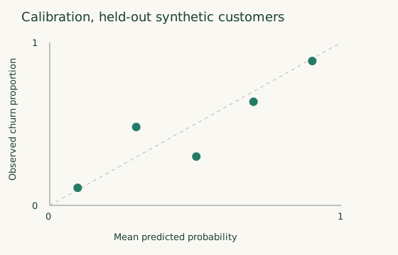
When cases predicted at 20% risk have the event roughly 20% of the time
Uplift / treatment effect
The change in an outcome caused by taking an action rather than its comparator
Propensity
The probability that the logging or assignment policy picks an action in a given context
Censoring
Follow-up ends before you know the event time, so the outcome is only partly observed
Elasticity
The percentage change in demand for a percentage change in price. A causal reading needs identification
Policy
A rule that selects actions from predictions, constraints and the available evidence
Overlap / positivity
The data include a chance of each action you want to compare, in the contexts where you would choose it
Off-policy evaluation
Estimating a new action policy's value from an older policy's logs. This needs suitable support, probabilities and assumptions
Contribution
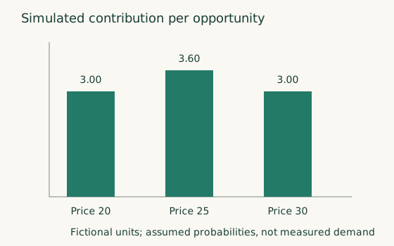
Revenue left after the costs defined for the decision, such as fulfilment, incentives and returns
Projects, in order of difficulty
What each one proves, and separately what makes it stand out. Those are different questions. The
Where you build it column names the chapter whose build exercise covers each project, or notes
when it is optional or spans several chapters.
#
Project
Where you build it
Proves
What makes it stand out
1
Deploy any pretrained model and get a public URL (3 hours)
Ch 5 warm-up (before two-week plan)
You can go from model to link
Nothing. It is a warm-up whose job is to remove the fear of deploying.
2
Structured extraction from messy text you have, into validated JSON
A modelling competition entry with a deliberately designed validation scheme (optional)
Ch 3 optional; Ch 7 Kaggle
You understand leakage and metric choice
The write-up, not the rank. "My first scheme was optimistic by 0.04 and here is why."
4
Scrape or pull a dataset that does not exist in tidy form, and publish the analysis
Ch 2
You can source your own data
Publishing the cleaned dataset so someone else can use it
5
A classical model served behind a real API, containerised and tested
Ch 3 build; Ch 6 hardening
The bridge from modelling to software
A load-test number, and a note on the accuracy-latency tradeoff you chose
6
Retrieval over a difficult corpus: statutes, versioned API docs, a codebase
Ch 5 (days 5–6 of two-week plan)
Retrieval quality, corpus design and evaluation
A hand-labelled retrieval set with recall at k for two chunking strategies
7
An evaluation harness as the product itself
Ch 5
Testing non-deterministic systems, which is rare
Publishing the failure taxonomy you found
8
A fine-tuned small model with a before-and-after table
Ch 5 optional
You know when fine-tuning is warranted
An honest four-way comparison, especially if the answer is "not worth it"
9
A workflow, not an agent, doing one real job for a real user
Ch 5
Architectural judgement
A written justification for not using an agent, with numbers
10
Reproduce a paper or core algorithm, then verify it
Ch 4 or Ch 7 Branch B
You can turn a paper into working code
Documenting where your numbers diverge, and why
11
A merged pull request in a major ML repository
Ch 7
Finding your way in an unfamiliar codebase, surviving review
Fixing a bug you personally hit while building something
12
A shipped product with real users who are not your friends
Ch 5 two-week plan + Ch 6
Scoping, distribution, operating under cost constraints
Baseline-relative quality with uncertainty, latency and operating cost
13
An open-source tool or dataset others depend on
Ch 7 Branch A capstone
Taste, engineering and stewardship
External adoption, which a reviewer can verify without trusting you
14
A rigorous public evaluation of something not measured well
Ch 7 Branch A capstone
Experimental design and statistical honesty
It is how individuals become known. Have someone review the method first.
15
A sustained record of shipping and writing up
Ch 8 (ongoing)
Durability, and that the rest was not a one-off
Eighteen months of dated write-ups cannot be copied
16
Offer, price or retention decision system with a reproducible evaluation
Ch 9; can supply Ch 7 capstone
Connecting prediction, intervention, constraints and feedback
An honest evidence report, no-action baseline and measured experiment when available
Three punch above their weight for the effort involved: the deliberate leakage write-up (project
3), the published failure taxonomy (project 7), and the honest fine-tuning comparison whose
answer may be "not worth it" (project 8). That last kind of negative result shows a tested
hypothesis and a fair decision. Explain the comparison, uncertainty and operating costs so a
reviewer can judge it.
Common pitfalls
Collected from practitioner writing and from resources that turned out to be dated when checked.
None of these are character flaws. Most are design problems with the material available.
About sequencing
Pitfall
Why it costs so much
Doing the maths before any code
The most common way people stall. If you are reading a maths book and have never written a training loop, the order is probably backwards.
Preparing for several roles at once
Five titles, five curricula, and none finished
Finishing courses without building
Video is enjoyable and does not transfer well on its own
Building evaluation tooling before reading traces
You end up measuring categories someone else invented for a different product
Waiting until you feel ready
Six months of courses with nothing shipped is worth less than one shipped, imperfect thing plus three months of courses
Resources that are commonly recommended and now dated
Resource
The issue
Better choice
nanoGPT
Marked "very old and deprecated" by its own author, whose README redirects readers
Excellent, and a month of material you will not use here
3Blue1Brown, then 18.065
Pre-transformer NLP courses
Fine as history, unhelpful as a current education
Transformer-first material
MCP tutorials from 2025
Protocol revisions can change lifecycle and transport assumptions. Older deployed versions may still be valid
Match the server/client version to the current specification and migration guidance
Technical traps
Trap
Why it matters
Data leakage
The most common technical mistake, and it never raises an error. It just improves your numbers.
Accuracy as the default metric
On a 1% positive dataset, "always no" scores 99%
ROC-AUC alone under heavy imbalance
Good ranking can coexist with poor precision. Add PR metrics, prevalence and performance at actual capacity.
A 0.5 threshold
A convention, not a decision
Reporting one number with no interval
Most beginner improvements are inside the noise
Trusting default feature importance
It misleads under correlated features, systematically
Changing three things at once
The result then teaches you nothing
Skipping the overfit-ten-samples check
Thirty seconds against several hours
Reading the transformer paper first
It introduces a 2017 encoder–decoder translation architecture. Learn attention with a small implementation first, then compare the paper with the architecture you use.
Reaching for a framework before writing the loop
You never learn the loop, and cannot debug it
An agent where a workflow would do
Non-deterministic, harder to evaluate, and more expensive
Fine-tuning as a source-update mechanism
Start with retrieval for facts that change, need citing or are private. Training does not enforce document permissions or keep sources fresh
Choosing a model by its leaderboard score
Benchmark construction and contamination can distort scores. OpenAI’s February 2026 audit cited both when dropping SWE-bench Verified; its July update also withdrew its earlier SWE-Bench Pro recommendation. Compare on your deployment task and protected holdout.
Kubernetes as a study project
Months of detour with little portfolio payoff at this point
"The customers table" as a data version
It changed yesterday
Response or churn risk treated as campaign benefit
Predicting an outcome does not identify how an intervention changes it
Predicting yesterday's selling price
It does not tell you which price improves profit
Unfinished labels treated as negatives
Delayed conversions, returns and churn corrupt the comparison
Optimising offers and prices independently
Combined discounts, contact fatigue and shared budgets can invalidate each policy's economics
About money and portfolios
Certificates mostly signal enrolment. Audit courses free and spend the money on compute.
Expensive cohort courses are often excellent, and their authors frequently publish most of the
same material free. Read the free version first.
Buying a GPU before exhausting free tiers is usually procrastination in physical form.
Ten shallow projects read worse than three deep ones.
Code you cannot explain is a real risk now that reviewers ask about repositories in detail.
Building in public works better in the quiet version: ship small things and write up what
broke. The high-profile examples usually had a large audience already.
Where thoughtful people disagree
This book takes positions throughout. These are the places where competent, experienced people
genuinely disagree, and where stating both sides is more impressive than picking one.
Question
One side
The other
Where this book lands
Top-down or bottom-up for deep learning?
Train something working first. Motivation collapses without early wins
Start from first principles, or you cannot debug a model that silently is not learning
Bottom-up first, top-down alongside, with the inversion offered for people who need the early win. It is a sequencing question, not a values one.
Does a beginner still need classical ML?
The jobs are in language models. You can be productive with an API
Interviews front-load it, and evaluating a generative system is the same discipline
Eight weeks, framed as the floor rather than the frontier
Frameworks or raw SDKs?
Stateful agents need durable execution and observability you would otherwise rebuild
Provider APIs converged, so the abstraction hides less than it costs
Both sides agree on the learning order: raw first
Retrieval or long context?
Long context can preserve relationships lost during chunking
Retrieval can reduce irrelevant context, enforce document access and control repeated input cost
Compare both, and a hybrid, on your corpus, tasks, permissions, latency and cost. No single context length is the right cutoff.
Agents or workflows?
Models improved enough that agentic loops now win on open-ended tasks
Most systems need clear steps and measurable outcomes
Workflow-first is safer for a portfolio, but be ready to defend it
Can you trust a model-based judge?
Ready-made metric suites let you start measuring immediately
Judges are useful only after error analysis has told you what to measure, and must be checked against human labels
Derive criteria from your own failures, then validate the judge
Have tabular foundation models replaced boosted trees?
Rankings change with model version, tuning and temporal/grouped deployment protocols
Compare trees, a suitable pretrained model and an MLP where warranted. See the version-specific evidence in Chapter 3.
Should learners use AI assistants?
They can explain unfamiliar code and support realistic engineering practice
Delegating a first attempt can bypass the understanding you meant to acquire
Protect independent attempts, then use assistance deliberately. Measure what you can still explain and build yourself.
Did AI cause changes in junior hiring?
AI could alter which entry-level tasks employers need
Macroeconomics, employer mix and changing seniority requirements also affect observed postings
Patterns in job-ad data do not settle causation. Plan with current local requirements and your own funnel.
Is Kubernetes required?
Job descriptions ask for it constantly
Serverless platforms let you ship real systems without it, and the hours are better spent elsewhere
Docker deeply, Kubernetes on the job. That is a side, and worth knowing you are taking it.
Keeping this book current
Three kinds of information in this book age fastest: prices and free tiers, model names and
capabilities, and salary figures. Treat any specific number as a snapshot, and check the source
before you rely on it.
The illustrated edition — 30 October 2026
The web edition adds shorter lessons, eight original interactive field notes, local search,
optional on-device reading progress, focus reading, a complete print edition and an
EPUB. Chapter Markdown is still the source for all of them.
Chapters 2–6 now include original worked examples, independent exercises, hints and explained
answers. Chapter 2 sets aside a holdout before you look at outcomes, and a shared causal primer
prepares the business cases. Completion gates ask to see your reasoning and debugging.
The reference lab supplies deterministic synthetic data, training-only
model fitting, separate calibration and test cohorts, a paired comparison, business decision
examples and filled reports. Its results illustrate a stated simulator and implementation, not
real commercial performance. The source inventory records cited URLs, without claiming that every
source was independently rechecked on the edition date.
Two studies shaped how the book asks you to work: Dunlosky and colleagues (2013), on which study
techniques actually hold up, and Roediger and Karpicke (2006), on why self-testing feels worse in
the moment and works better in the end.
A few places deserve extra scepticism, and I would rather point them out myself. Causal and
experimental methods rest on assumptions about assignment, confounding and interference.
Chapter 9 now states those assumptions for the
business cases and adds primary sources. The two-mode rule for AI assistants is a reasonable
compromise, not a proven method. And the four-to-eight-month job-search allowance is a planning
judgement, not an outcome estimate.
If something here has drifted out of date, that is the field doing what it does. Check it against
the source, adjust, and keep going. If you find a broken link or a claim that no longer holds, an
issue or a pull request on this repository is very welcome. Corrections from readers are how a book
like this stays useful.
What changed in the illustrated edition review
Edition 2026.10.1. Every diagram in the PDF now prints in its own place, and the EPUB passes
the EpubCheck validator that ebook stores use.
One thread, end to end. Chapters 4 and 5 now start with a same-thread build, and Chapter 6
runs the Chapter 3 model alongside the Chapter 5 application. Chapter 7 shows how each
capstone stays connected, and Chapter 8 adds operations evidence to the portfolio template.
New practice. A broadcasting exercise in Chapter 2, a training-debugging checklist in
Chapter 4, document field extraction and output guardrails in Chapter 5, and explained exercises
in Chapters 6, 8 and the offer, price and churn guides.
Production. Safe artifact loading, provider outages, retention and erasure, and incident
severity with blameless write-ups.
Laboratory. Stricter manifest and sample-ratio checks, an experiment result reported with its
uncertainty, and a test that the checked-in reference matches a fresh run.
Corrections. Consistent fine-tuning placement, hour figures and reading selections. Missing
links and resource notes added. A citable edition with EPUB and PDF downloads.
Web edition. Illustrated plates for the start page, reader's guide, applied guides and lab
reports. Full-width field notes in the lab. Dollar amounts no longer render as mathematics.
Licence. The text, illustrations and lab reports are now CC BY 4.0, so you may share,
translate and adapt them with credit. The website and code remain under the MIT licence.
What changed in the October 2026 research revision
Business cases. Added Chapter 9 with detailed offer, pricing and churn guides, conditional
model recommendations, worked economics, practice data and production delivery gates.
End-to-end coverage. Added rules for feature availability, label maturity and outcome
observation, plus calibration and test discipline, regression and forecasting, optional
segmentation and anomaly methods, experiment protocols, model lifecycle and delayed-outcome
feedback. The business guides separate competing events, the uncertainty of picking the
best-looking policy, and joint or adaptive assignment.
Current evidence. Reviewed 2026 tabular, causal, survival, recommendation, pricing and agent
research. Recent preprints appear as conditional challengers, with criteria for reproduction and
adoption, not as universal winners.
Corrections. Updated library compatibility, course editions, contribution policies and hiring
data. Qualified benchmark claims by model variant and sampling protocol. Strengthened
guidance on leakage, uncertainty, permissions, release evaluation and rollback.
Sources. Primary papers and official documentation are linked where the chapters use them,
with assumptions and practical limits alongside model recommendations.
What changed in the September 2026 revision
For readers already partway through, these are the changes worth knowing:
Setup. Python 3.14 in the setup commands, and a note on uv's new default project layout
(Chapter 1).
AI assistants. A 2026 randomised trial on learning with an assistant, and a two-mode rule
adjusted to fit it (above).
Short new sections. Reasoning-effort costs and agent skills
(Chapter 5), regulation as part of production
(Chapter 6), and a security reference for the AI Engineer branch
(Chapter 7).
Tabular models. A more careful picture of tabular foundation models against boosted trees
(Chapter 3).
The job search. Newer hiring and pay data, and interviews that now include an AI assistant
(Chapter 8).
Resources. Chapter 5 now points to Anthropic's free Claude Academy course, one course website
no longer loads, and many notes were refreshed for new versions, prices and owners.
A note from the author
I have spent my career as a developer, moving between domains, and every move brought a new set of
challenges. Through all of them, one habit has helped me more than any tool: starting from a
roadmap. A good roadmap does two quiet things. It builds the foundation in the right order, and it
teaches you to think in systems — to see how the pieces connect before you start collecting them.
This book is that habit written down, for the move I think matters most right now: from software
engineering into AI and machine learning.
I want to be open about how it was made. I used AI models, including Fable 5, to help me research
and draft it. The plan, the judgements, and the final words are mine, but it felt right that a book
about working with these systems should be honest about being written with their help.
I am not only the author here. I follow these chapters myself, to refresh my own skills, because in
this industry the learning never stays done. If you find something that has aged, treat it the way
this book will teach you to treat every claim: check it, correct it, and keep moving.
The short version. Choose a target role, a weekly time budget and a working Python environment.
Start on your own CPU or a free notebook service. You finish with a repository another person can
run, and no hardware to buy.
About eight hours. Do the days in order, and finish every step that ends in a commit or log line.
Day
Hours
Do this
Done when
1
2
Read "Pick one target role" below. Write your choice, one non-salary reason and a weekly study budget in README.
Role, weekly hours and study sessions are written down
2
2
Run the uv commands below. Commit the project and push to a repo.
Fresh clone passes the locked install and import check below
3
1
Create LOG.md. Add today's line (see What to build).
First log entry exists
4
1
Open Google Colab. Run import pandas as pd; print(pd.__version__). Try switching to a GPU runtime.
Notebook runs; CPU is fine today
5
2
Read Eugene Yan's interview article (linked in Resources) and note the two skills in bold. Check five current job descriptions in your target market and skim the compute table.
Role choice matches real requirements. You have a CPU plan and an optional GPU plan
What you will be able to do
Name the specific role you are working towards, and open a project without fighting your tools.
A quick entry check
Try these with documentation but without a tutorial. They show what to prepare, and are not a timed
admission test.
Read a small CSV, check that an amount is numeric, and return a useful error for a bad row.
Write a function and a test, run them from a terminal, and explain the stack trace of a
deliberate failure.
In a throwaway repo, make a Git commit, look at its diff, and undo one accidental change.
Explain why 12 events among 80 eligible cases is 15%, then say what would make that denominator
wrong.
If the first three feel unfamiliar, use the programming resources in
Chapter 2's resource list before
counting the chapter budgets. Take one Python course, such as
CS50P
or Python for Everybody,
then Learn Git Branching and
The Missing Semester
for Git and the shell. If fractions or function notation feel rusty, list the maths topics to
revisit and work through the examples alongside Chapters 2 and 3. You can start without a full
mathematics course. The reference lab is a small project with no API calls for
checking your local workflow.
What to learn
Pick one target role. The five common titles look similar from outside and lead to quite
different curricula. Trying to prepare for all of them at once is one of the more common reasons
people stall. Treat the table as a guide to the work. Employers use these titles inconsistently.
Role
What the day looks like
Qualifications to check in actual vacancies
Fit for a developer
AI Engineer
Products using foundation models: context, tools, retrieval, evaluation, cost and latency
Software experience and product judgement. Degree filters vary
Application skills transfer directly
ML Engineer
Data pipelines, training, serving and scaling. Model performance under deployment limits
Proven software and statistics skills. Degree filters vary
Good, with more statistics and systems work
Data Scientist
Experiment design, causal questions, metrics and communicating decisions
Statistics, domain knowledge and sometimes a quantitative degree
Good, with the most statistics
Applied Scientist
Research alongside production code
Some employers require a graduate degree or equivalent research experience
Needs a stronger record of experiments and research
Research Engineer
Frameworks, distributed training and implementing new methods
Systems ability and research experience. Publications and graduate degrees depend on the role
A demanding route for developers with relevant systems experience
Data Engineer is worth considering as well: ingestion, data quality, modelling, orchestration
and reliable analytical systems. Your SQL, backend and infrastructure experience can transfer.
If you cannot decide, AI Engineer is a reasonable first choice for someone who already ships
applications. Revisit it after checking local vacancies and after your first project. A
title alone does not show hiring demand or an employer's degree requirements.
Know what interviews can assess. Eugene Yan has published
his own hiring rubric. He assesses software
engineering fundamentals, data literacy, comfort with uncertainty, evaluation frameworks,
and breadth of knowledge. It is one practitioner's rubric, so expect other interviews to differ.
The projects in this book are built to show the two skills in bold.
Set up your tools. Use one documented workflow, and check version-sensitive examples against
current documentation.
Environments: use uv. It manages dependencies, virtual
environments and Python installations. First follow its
installation instructions for your operating system,
reopen your terminal if needed, and check uv --version. Then create the project:
uv run --locked python -c "import numpy as np; import pandas as pd; print(np.__version__, pd.__version__)"
Both version numbers should print without an error. Open notebooks with
uv run jupyter lab. Commit pyproject.toml, uv.lock, .python-version and the generated
src/ package. Note the Python patch version, uv version and operating system. Use
uv sync --locked and uv run --locked ... for a reproduction check. The flag fails if the lock
disagrees with project metadata, rather than quietly changing it. See
locking and syncing. A lock does not pin your
data, GPU driver or every hardware-dependent result.
Two details trip people up. Since uv 0.12, uv init creates a small package under src/, which
suits the tested cleaning functions you write in Chapter 2. Add --no-package if you want the
older single-file layout. For the Python version, pick the newest one that PyTorch, the
deep-learning library you meet in Chapter 4, has ready-built packages for. In September 2026 that
is 3.14, as the official
PyTorch installation guide shows. If a needed library
lacks a compatible wheel, choose a supported Python version and regenerate the lock on purpose.
pandas 3.0 changed some defaults. Copy-on-Write is now the only mode, so chained assignment
cannot update the original dataframe. Use a single .loc[...] = ... assignment. Text columns also
default to a string dtype. Some operations still support inplace=True, so seeing it does not
date a tutorial. Check the
pandas migration guide. NumPy's
old aliases such as np.int, np.float and np.object expired in
1.24. NumPy
2.0 reintroduced np.bool with boolean
dtype semantics. Use explicit dtypes when precision matters.
Editor. VS Code with the Python and Jupyter extensions is a practical default. Select the
project's .venv interpreter and notebook kernel. Its
data science tutorial
also covers conda and TensorFlow. Those are valid, but use one documented environment here.
A note on package sources. At work, follow your organisation's package and licensing policy.
Anaconda's commercial terms depend on the service and organisation, so read its current terms if you
use it. Miniforge with conda-forge is another option if you need conda.
Where your compute comes from.
Nothing on the main path of this book needs a GPU you have to buy. "I cannot learn deep learning
without a GPU" is a common worry and, happily, not true.
Option
Cost
Good for
Worth knowing
Your computer
No additional service cost
Chapters 1–3 and small CPU experiments
Keep the dataset small and note memory use and runtime
Google Colab
Free tier
Quick interactive notebooks
GPU type, availability and limits change. Save work and checkpoints outside the runtime
Kaggle Notebooks
Free tier
Public datasets and notebook experiments
Check account eligibility, the current accelerator allowance and session limits
Lightning AI
Free tier or credits where offered
Persistent development projects
Check which machines use credits and how saved work is billed
Modal
Starter credits, then usage charges
Scripted CPU/GPU jobs and services
Credits and endpoint billing follow different rules. Set a spending limit and check current pricing
Start locally or in a free notebook. Choose a GPU service later, to fit the exercise's memory,
runtime and storage needs. A provider's allowance can change, so keep a CPU fallback and checkpoint training
so it can resume. Official compute links are in this chapter's resources.
Resources
All 13 resources for this chapter, with notes on each, are in resources/.
Create your learning repository, add a LOG.md, make your first commit, and push it. Public is
better, even this early. One line per session is enough:
2026-10-09 · 2h · Created repo with uv; CPU notebook runs · Broke: selected wrong kernel
From a fresh clone, run uv sync --locked, then repeat the import check above. Write those exact
commands in the project README, with your role and weekly study sessions. Keep credentials and
private datasets out of the repository. A public project helps when its data and code can be shared.
Before you move on
You can state the role you are training for, and one reason for it that is not salary.
Your weekly hours and study sessions are written down. If ten hours a week is unrealistic, stretch
the schedule.
A fresh clone installs from the committed lock and passes the documented import check.
You can correct a pandas chained-assignment example using the migration guide.
You have a working CPU environment and know how to check an optional GPU service's current limits.
Certificates. A certificate shows you finished a course, not that you can build or evaluate
things on your own. Historical MOOC completion rates count everyone who registered, including
people who never meant to finish, so they are a poor guide to your own success. Alongside any
certificate, build something a reviewer can inspect.
Perfecting the plan. It is possible to spend a happy weekend on a study schedule. The schedule
is not the work.
The short version. You already program. This chapter teaches the data dialect — arrays and
shapes, dataframes and cleaning judgement, and enough SQL to be trusted with real data. You finish
by publishing a small, reproducible analysis of a dataset you found yourself, which becomes the
seed of everything you build later.
This dataset carries forward. Chapter 3 models it. Chapter 5 can use documents in the same
domain. Keep the domain where you can. Document a needed change, rather than forcing an unsuitable
dataset to support a claim it cannot answer.
Choose a dataset you can finish
Before investing in cleaning, check five things:
Permission: you may download, analyse and publish the intended examples.
Grain: you can say what one row represents and spot duplicates or repeated entities.
Question: one useful descriptive question and a feasible binary or numeric prediction target.
Clocks: you know when inputs would be available and when outcomes can be seen. A current
export with no history supports a limited exercise, not a verified historical backtest.
Size and continuity: a small sample runs on your machine, and related public documents could
support the later application.
If choosing stalls, use the reference lab while looking for your own portfolio
dataset. It uses synthetic data, so its results show behaviour under stated assumptions. A city
open-data export, a permitted export of your own data, or a small transaction dataset can work if it
passes these checks. An ordinary, modest dataset is enough.
Set aside the test set before you explore outcomes. As soon as you know what you want to
predict, write down the prediction time and time or group split, and set aside the final
holdout. All-row checks of source, schema and integrity are useful. Learned transformations,
charts that use the target, and feature choices belong on training and development data only. If
you have already explored every outcome, label that work exploratory and find fresh data to confirm
it. Splitting afterwards does not undo what you have seen. Chapter 3 reviews this design.
About ten hours a week. Each week ends with something on GitHub.
Week
Focus
Do this
Done when
1
Setup + NumPy
Reuse the uv project, shortlist your dataset, learn NumPy basics, start Essence of Linear Algebra
arr.shape and broadcasting exercises work
2
pandas
McKinney ch 4–8, 10 or pandas Getting Started. Write 3 cleaning functions with tests
Functions in src/ and tests in tests/ pass
3
SQL
SQLBolt basics, selected ThoughtSpot window and join lessons, then DuckDB on your CSV
Top-N-per-group query and join-cardinality check run
4
Your dataset
Confirm data you sourced. Write a schema/source manifest and cleaning decision log
Eight+ meaningful checks pass. Log has 3+ decisions
5
Publish
README with question, answer and limitation. Charts that answer questions. A locked fresh-process run
A stranger can clone and reproduce it
New words in this chapter, such as array, broadcasting, dataframe and point-in-time, are explained
where they first appear below and collected in
Terms in plain English.
Work in the Chapter 1 project. Add the SQL, plotting and test dependencies, then commit the changed
project files:
uv add duckdb matplotlibuv add --dev pytest
After writing the Week 2 tests in tests/test_*.py, run uv run --locked pytest from the project
root. Use pytest's getting-started guide
for discovery and assertions. Start the linear-algebra videos with chapters 1–4, ending with
"Matrix multiplication as composition". Later lessons are optional, inside the same 50-hour budget.
What you will be able to do
Take a messy dataset you found yourself and turn it into a published, reproducible analysis that a
stranger can run with one command.
What to learn
Worked lesson: the event happened, but you did not know it
Suppose you predict at the start of 3 January, using the previous seven days. These invented
transactions separate when an event happened from when the service received it:
Amount
Event time
Available at
Available for this prediction?
10
1 January
1 January
Yes
20
2 January
4 January
No: it arrived later
30
4 January
4 January
No: the event is in the future
The historical total is 10. Filtering on event time alone gives 30 and leaks a late arrival.
Using today's complete customer total gives 60 and also includes a future event. Values correct
today can be wrong inputs for a past decision.
from datetime import datetime, timedelta, timezonedef day(number): return datetime(2026, 1, number, tzinfo=timezone.utc)events = [(10, day(1), day(1)), (20, day(2), day(4)), (30, day(4), day(4))]as_of = day(3)total = sum(amount for amount, event_at, available_at in events if as_of - timedelta(days=7) <= event_at < as_of and available_at <= as_of)assert total == 10
Try it yourself. Move the decision to 5 January. Which records now qualify, and what is the
total? Then add an event exactly at the prediction time. Decide whether it belongs before running.
Hint and explained answer
Both clocks must pass. At 5 January all three original records qualify, so the total is 60.
An event at exactly as_of falls outside the half-open event window [as_of - lookback, as_of).
That boundary stops the current decision's own activity from becoming its historical input. The
availability rule here does include records arriving exactly at as_of. Test and document whether
your real extraction order can actually use them.
Use this tiny fixture to test a larger SQL or pandas implementation. The
reference lab builds the same habit on a reproducible synthetic project.
Core concepts
Thinking in arrays. You are fluent in loops. Machine learning is written in shapes and batches,
and the second dialect takes a little while. What you need is small but you need it cold: shape
and dtype, indexing and slicing, views against copies, reshape and transpose, axis semantics,
vectorising a loop into an array expression, and above all broadcasting.
Broadcasting deserves the extra time. It is the set of rules by which NumPy stretches a smaller
array to match a larger one's shape. A large share of the debugging you will do over the next six
months is shape errors, silent broadcasts and transposes in the wrong place.
Try it yourself. Predict errors.shape before running it. Every prediction equals its target,
so the mean squared error should be zero. What does (errors ** 2).mean() return, and why?
Hint and explained answer
Align the shapes from the right. (100,) is treated as (1, 100), and each size-1 dimension
stretches to match. So errors has shape (100, 100): every prediction minus every target. The
mean is 1666.5, the average squared difference over all 10,000 pairs, and nothing raises an error.
Compare matching rows with predictions[:, 0] - targets, then assert errors.shape == (100,)
before reducing. That one line catches the same bug in a metric, a loss or a pandas-to-NumPy
conversion.
Alongside this, watch 3Blue1Brown's
Essence of Linear Algebra.
Three hours of video, and it gives you one idea that pays off immediately: a matrix is a
transformation of space, not a grid of numbers to row-reduce. After that, "a layer is a linear map
followed by a nonlinearity" stops being jargon. It helps to pair each chapter with code, though.
It is quite possible to finish the series feeling enlightened and still be unable to compute a
matrix product.
Thinking in tables. pandas, and the judgement that goes with it. The library is the easy half.
Alongside your notebook, record every cleaning decision you made, what you rejected, and how the
choice would change a model downstream. Here is an example decision log, with invented
percentages:
## delivery_time — 8.2% missingPattern: missingness correlates with carrier == "regional" (34% missing) against 0.4%for national. This is not missing completely at random: it depends on observed carrier.This pattern alone cannot establish MAR versus MNAR; missing delivery times are unobserved.Rejected: mean imputation. It would smear the national distribution across regional rows and hide the fact that we simply do not observe this segment.Rejected: dropping the rows. It removes 8% of the data, and non-randomly.Chose: keep the nulls and a delivery_time_observed flag for descriptive coverage checks. Report observed timing by carrier, alongside missingness and sample counts.Impact: observed rows alone cannot establish timing for all regional-carrier deliveries.
That paragraph is the thing worth showing people. Anyone can call dropna(). The judgement is the
scarce part, and it maps directly onto "data literacy" in a hiring rubric.
The author-hosted missing-data chapter explains why
dependence on an observed field can fit MAR (missing at random), and why MNAR (missing not at
random) needs sensitivity analysis.
Separate missing features from missing targets. If delivery time is the Chapter 3
target, its eventual value and observed flag cannot be predictors at dispatch. Avoid filling an
unfinished target with zero or a mean. A package still being tracked has a right-censored
duration: you know how long it has gone undelivered, not when it will arrive. Evaluating only
completed deliveries can leave out the slowest ones. The
scikit-survival introduction
explains event indicators and censoring. A survival model is optional depth, not an extra
prerequisite. For a first project, a fixed-horizon target such as “delivered within seven days” is
often easier to define. After seven days, a tracked non-delivery is negative. A lost tracking
record is still unknown. State which population and follow-up your evaluation covers.
For a feature available before prediction, compare an imputer and missing indicator fitted inside
the training pipeline with a model that handles that feature's missing values. Either way, keep the
raw missingness information in your analysis.
SQL. Grain, joins and aggregation carry across tools, though syntax and NULL behaviour vary by
engine. Get comfortable with CTEs, window functions (ROW_NUMBER, RANK, LAG, running totals),
join cardinality, and point-in-time correctness.
That last one matters more than it sounds. Most serious data-leakage bugs in machine learning are,
underneath, a query that accidentally used the future.
If an assistant writes SQL, check it against a schema you understand and a tiny table with
duplicates, NULLs and boundary dates. Plausible SQL can give the wrong denominator with no error.
A schema is more than column names. Define dtypes, units, allowed categories and what a missing
value means. Keep leading zeros in identifiers. Choose a timezone policy. Store money with a
documented currency and rounding rule. Tell apart a zero, an unknown value and a value that does not
apply. Recheck pandas string and nullable dtype behaviour after upgrades. In pandas 3.0, default
string storage uses PyArrow when installed and falls back otherwise, as the
string migration guide
explains.
Write the expected join cardinality before joining. One customer with three orders and four
support events produces twelve rows if both event tables are joined directly. Summing the joined
orders inflates revenue fourfold. Aggregate each event table to the intended grain first. In
pandas, use validate="many_to_one" for a unique customer lookup and indicator=True to check
unmatched rows. Its
merge documentation also warns
that NULL keys on both sides match each other, unlike usual SQL joins. Test this explicitly.
Write a data contract before training. Name the unit of a row, its unique key, the prediction
time, the feature lookback, the outcome window, and when that outcome becomes complete. Keep both
event_time (when something happened) and available_at (when your service could first use it). A
transaction from Monday that arrived on Friday was unavailable to Tuesday's model. Historical
features must pass both clocks, and later corrections need version history.
Feast's point-in-time joins
show historical retrieval. Check how your own query and tool handle availability time.
Some public exports hold only a current snapshot, with no availability history. Record that limit,
and avoid inventing timestamps or claiming a verified backtest. Test your join logic with small
synthetic late-arrival cases, and choose a Chapter 3 split your data can support.
For a customer snapshot at time t, build features from [t - lookback, t), using records
available by t. Build labels from the outcome window that follows. An unresolved outcome is
unknown, not a negative. Record label_available_at and outcome_observed separately from the
planned maturity date, because a window can pass while its source ledger is still incomplete. At a
simulated training cutoff, use only labels that the observation window, reporting delay and actual
availability allow. Report missing outcomes by cohort and exclusion reason. Elapsed time alone does
not prove follow-up is complete.
Test unique keys, join row counts, timezone conversion, missingness, late arrivals and duplicate
events. Store the extraction cutoff and source version with the data. Record permission to use
the data, keep customer identifiers out of public examples, and publish only data whose licence and
permissions allow it. When the original data is private, a reproducible synthetic example is enough.
Reproduction needs a data manifest. Record the source URL or export/query version, licence,
retrieval date, extraction cutoff, raw-file checksum, schema version, code commit and environment.
Where permitted, keep raw inputs unchanged. Document any sampling, seeds and exclusions, and use the
same population denominator in your text and charts. Run the cleaning and analysis in a fresh
process with the locked environment, not from the notebook's execution history. The questions
in Datasheets for Datasets help explain who is represented and
which future uses the dataset cannot support.
If raw data is not in the repository, include its exact download or export steps and expected
checksum. If the documented input is missing or differs, the analysis should fail clearly, not
quietly analyse a newer export.
Resources
All 31 resources for this chapter, with notes on each, are in resources/.
uv — official documentation — Astral maintainers. Free
documentation, 2–4 hours. Getting Started and Projects are enough.
These are whole-resource estimates, and some are alternatives, so do not add them up. Fit selected
chapters and lessons inside the 50-hour project budget, and finish the analysis before optional
depth.
If Python is not yet one of your languages, do CS50P first. Its
90 to 120 hours sit on top of this chapter's 50, not inside them, and the chapter will make much
more sense afterwards.
What to build
A published data product. A public repository containing:
A README stating the question in one sentence, the answer in one sentence, and the limitation in
one sentence
pyproject.toml, uv.lock, Python/platform details and a command tested after uv sync --locked
A src/ package with your cleaning functions, not just a notebook
At least eight meaningful checks spanning cleaning functions, unique keys, joins, timestamps and
missingness
Your cleaning decision log
Only charts that answer named questions, each with a denominator, units, source and limitation.
Cover the relevant distributions, missingness/coverage and time or group variation. Show
uncertainty when making an estimate. Use readable labels and a palette that works without colour.
A data contract covering row keys, both timestamps, feature windows, label maturity, actual
outcome availability/coverage and permitted use
A source manifest with raw-input checksums, extraction cutoff and documented exclusions
Give the package an analysis entry point and document its exact uv run --locked ... command. It
must read the documented inputs and rebuild the cleaned output, summary results and chosen charts
without notebook state. Run uv run --locked pytest separately. Passing tests alone do not
reproduce the analysis.
Choose a dataset that you found yourself: a city open-data portal, a government export, a niche
marketplace, or your own data exported from a service you use. Before Week 4, pick an outcome you
could later predict, such as a delay, a price or a category, and the inputs available at
prediction time. Chapter 3 will ask you to model
it. In the handoff, state the prediction time, row/group key, reserved holdout and a workable split.
If the dataset cannot support a supervised question, change the dataset and write down why. Avoid
inventing labels or using the outcome as an input.
Before you move on
A stranger can install the locked environment, run the tests and regenerate your analysis with the
documented command.
You can defend two cleaning decisions against "why not just drop those rows?"
You can write and explain a top-N-per-group query, checking ties and duplicate keys on a fixture.
Documentation is allowed.
You can predict the output shape of a broadcast before running it.
You can show that a late-arriving record and an unfinished label cannot enter a training row.
You can tell apart a mature observed negative, a censored duration and a missing outcome, and
explain how each enters your denominator.
You can show that a join preserves the intended grain and explain the denominator of each chart.
The Chapter 3 handoff names a target, prediction time, available inputs and defensible split, and
states any historical-data limits.
A few things worth knowing
The free Python Data Science Handbook at jakevdp.github.io is the 2016 first edition,
written against Python 3.5, though still widely recommended. The NumPy and matplotlib chapters are
useful for the concepts. The pandas and scikit-learn chapters teach idioms that may now raise
errors or behave differently, so check its examples against current documentation. McKinney's
book plus the pandas migration guides is the main route here.
Polars is optional. This chapter uses pandas to match its selected tutorials. Polars is a
useful alternative when your team's stack or measured memory and runtime needs call for it.
scikit-learn supports Polars transformer output.
Rewrite one cleaning function only after the analysis works, and check correctness before speed.
Titanic, Iris and MNIST are fine for a ninety-minute warm-up. As portfolio pieces they are so
common that they tell a reviewer very little about you, which is a shame given the effort. A
dataset you sourced yourself does much more work on your behalf.
The short version. This chapter teaches you to train a model carefully. Split the data so the
score means something, pick a metric tied to a real cost, compare against a simple baseline, and
explain the result. The same habits carry straight into evaluating language models later. You
finish with a model served behind an API.
Use your Chapter 2 dataset. Same repo or a fork — the story should connect. Review the holdout
you set aside when choosing what to predict, and keep it fixed after seeing outcomes.
About ten hours a week. Follow the rows in order, including the baseline and the README.
Week
Focus
Do this
Done when
6
Problem + split
Recheck the target and reserved split (random / time / group). Justify it before fitting
README records the split and earlier exploration
7
Baseline + leakage
Prior-probability baseline (DummyClassifier). Leak preprocessing on purpose, then fix it with Pipeline
Before/after scores in README
8
Logistic regression
ISL or scikit-learn MOOC. Pick a metric tied to cost
Beats the baseline, or explains why to keep the baseline
9
Trees
Random forest + one boosted tree. SHAP on one wrong prediction
Quality, calibration, runtime/memory and latency compared
10
Calibration + threshold
Reliability plot on held-out data. Tune the decision on validation costs
Can explain probability and threshold separately
11
API
FastAPI /predict with Pydantic validation. Test a valid and an invalid request
Served predictions match saved bundle. Bad input returns 422
12
Polish
Confidence intervals, a "what failed" section and a load-test note
README is the deliverable
13
Buffer
Rebuild one model from an empty file. Practise your leakage story for interviews
Can rebuild without a tutorial
The table uses binary classification as its first-project example. For a numeric target, use
DummyRegressor, regularised linear regression, RandomForestRegressor and a boosted regressor.
Swap the threshold exercise for error/interval analysis and a cost-based decision rule. The same
split, holdout and API requirements apply. A well-explained negative result completes the
comparison. Avoid searching for a misleading split just to beat the baseline.
For a first multiclass project, compare a class-prior baseline. Report a confusion matrix and
per-class precision/recall alongside the aggregate you chose. A binary cost threshold does not carry
over to several classes. Define the cost of each action/outcome pair and choose the lowest expected
cost using suitable probabilities. Multilabel tasks also need their own label-level decision and
evaluation design. Leave them for later if the basic workflow is new.
In your uv project, start with uv add scikit-learn. In Week 9, add the boosted-tree and SHAP
packages you chose, following their official install guides, and commit the updated lock. Keep one
boosted candidate. Installing three libraries is not a model comparison.
Is this still worth eight weeks in 2026?
Yes. The skills here support both tabular business decisions and generative systems. A more capable
pretrained model still needs a deployment-matched test, a baseline, a suitable metric and a
cost-aware decision. The split and leakage habits carry into
Chapter 5, though agent evaluation also needs its own tests for
tools, safety and interaction.
Eight weeks, then, rather than six months.
What you will be able to do
Take an unfamiliar dataset, choose a validation scheme and defend it, choose a metric and tie it to
a real cost, compare to a simple baseline, and explain in writing why each model helped or did not.
What to learn
Worked lesson: a probability is not an action
Four made-up development cases have predicted event probabilities [0.1, 0.4, 0.7, 0.9] and true
labels [0, 1, 0, 1]. A false positive costs 2 units and a false negative costs 8. Assume correct
decisions have zero cost and there is no capacity limit.
At threshold 0.5, the last two cases are positive: one false positive and one false negative cost
2 + 8 = 10. At threshold 0.2, the last three are positive: one false positive costs 2. The model
has not changed. The action policy has.
With calibrated probabilities and these costs, compare the cost of acting, 2 × (1 - p), with the
cost of not acting, 8 × p. Acting is cheaper when p > 2 / (2 + 8) = 0.2. Set a rule for ties.
This assumes the error costs describe the decision. It cannot show a treatment benefit from a
churn-risk score.
probabilities = [0.1, 0.4, 0.7, 0.9]labels = [0, 1, 0, 1]def observed_cost(threshold, false_positive_cost=2, false_negative_cost=8): return sum(false_positive_cost if p >= threshold and y == 0 else false_negative_cost if p < threshold and y == 1 else 0 for p, y in zip(probabilities, labels))assert observed_cost(0.5) == 10assert observed_cost(0.2) == 2
Try it yourself. Swap the costs: false positives cost 8 and false negatives cost 2. Work out
the threshold and its observed cost. Is a four-case table enough to show calibration?
Hint and explained answer
Compare 8 × (1 - p) with 2 × p. The threshold is 0.8. Only the 0.9 case is positive, so the
0.4 case is a false negative and the total observed cost is 2. Four cases cannot show reliable
calibration or a lower cost in production. Set the rule on development data. Then evaluate the
frozen model, calibrator and policy on independent data, with suitable uncertainty.
The reference lab has a reproducible baseline comparison. Write down your
expected result before running it, and explain any difference from what you see.
Core concepts and practical failure modes
On a first pass, focus on the split, baseline, pipeline, metric and decision. The dated benchmark,
advanced uncertainty and causal sections below are optional depth after that baseline works.
The learning problem. A model maps inputs to outputs, and a loss measures its errors. Many
models optimise differentiable parameters with gradient-based methods. Trees learn partitions, and
linear regression can also use a direct solver. Learn regularisation, bias and variance, and how
each candidate is optimised. Not every model trains like a transformer.
Learning curves are the most practically useful idea here and the most often skipped. Plotting
training and validation score against training-set size helps you judge whether more representative
data or a different model might help. Treat it as a clue to test, not a firm diagnosis. Label noise,
distribution shift and a changing population mix can produce similar patterns. Keep time or group
structure while building the curves.
Validation, which is where the real care goes. Your validation score estimates performance under
its sampling and deployment assumptions. Information not available at the simulated training or
prediction time can quietly invalidate it. Leakage often makes scores look too good, and even a
clean holdout cannot promise performance after an untested change.
Three families to know:
Kind
What happens
Guard
Preprocessing leakage
You fit a scaler, imputer or target encoder on the whole dataset before splitting, so every fold has seen the test set's statistics
Put all preprocessing inside a Pipeline, so cross-validation refits it per fold
Temporal leakage
You use information that did not exist at prediction time. Random K-fold on time-ordered data trains on Thursday to predict Wednesday
TimeSeriesSplit, or rolling-origin backtesting
Group leakage
Rows from the same entity land on both sides of the split, while you claim performance on unseen entities
GroupKFold or StratifiedGroupKFold for that deployment question
Two questions, asked before you choose a splitter, prevent most of this: does a row's identity
repeat, and does time matter?
Match the split to deployment. Predicting next month's activity for existing customers can fairly
reuse their earlier histories. If the launch includes new customers, also evaluate on unseen ones.
A time split and a group split answer different questions, and sometimes you need both. Leave out
immature training labels. If a label needs 30 days plus seven days of reporting delay, those 37 days
must have passed by the simulated training cutoff. A fixed row-count gap in TimeSeriesSplit does
not by itself enforce a calendar-based label window.
Keep separate training, model-selection, calibration/decision-selection and final test data, or
use carefully designed out-of-fold estimates. Refitting a model can change its calibration, so
evaluate the exact model and calibrator you will serve. Early stopping, feature selection,
resampling and hyperparameter tuning all belong inside the training procedure. Open the final test
only after the choices are frozen.
Label maturity and observation are separate checks. A 30-day window can end with the source record
missing. Keep that out of the negatives, and avoid quietly scoring only the matched outcomes. Report
coverage by time and cohort, and say which population the score represents. A duration target with
incomplete follow-up needs a censoring-aware design, as
Chapter 2 explains.
A pipeline is necessary, but it does not choose the right time or group handling for every
component. For example,
scikit-learn's TargetEncoder
uses cross-fitting in fit_transform. Calling fit(...).transform(...) on the same training rows
does something different. Default internal folds are random. Since 1.9 you can pass grouped
splitters through metadata routing, but every row must appear in a validation fold exactly once. An
ordinary forward-only TimeSeriesSplit breaks that rule. Time-ordered encodings need an explicit
past-only design or a different encoder. Keep a training row's own and future labels out of its
feature encoding.
Repeatedly picking the best score across many models and settings also overfits validation. Use a
fixed tuning budget and an untouched test. To estimate the whole selection procedure, use
deployment-matched nested validation. Compare models on the same rows and horizon, and record
version, seed, search budget and failed runs. The
nested-CV example
explains the selection bias, but its random folds need adapting for time or groups.
Metrics, which are decisions in disguise. On a dataset with 1% positives, a model that always
predicts "no" scores 99% accuracy. A metric is a claim about what it costs to be wrong, and choosing
one is a business decision you are making on someone's behalf, usually by leaving it at the default.
Use
DummyClassifier(strategy="prior")
as the probability baseline. It estimates class frequencies from training labels and predicts
the majority class. Unlike strategy="most_frequent", its probabilities are not forced to zero and
one, so it is a useful log-loss/Brier comparator. Also report the simplest real action policy under
your stated costs, such as always taking no action. A probability baseline and an action baseline
answer different questions.
Learn precision and recall well, and when each matters more. ROC-AUC measures ranking, but can
coexist with poor precision when positives are rare. Report average precision or a clearly defined
PR-AUC, positive prevalence, and precision/recall at your team's real capacity. PR metrics also
depend on prevalence, so they are not directly comparable across datasets.
Probability and action are separate. A score of 0.8 should mean about 80% positives among
similar scored cases. Check a reliability diagram and log loss or Brier score. Those losses also
reflect discrimination, so neither alone proves calibration. Fit sigmoid or isotonic calibration on
independent, representative data and recheck it by cohort. Small calibration samples make flexible
isotonic fits unstable. Calibration on last month's sample does not guarantee calibration after
prevalence, eligibility or data collection changes.
scikit-learn's calibration guide
explains the methods. Choose thresholds on validation data using costs and capacity, then evaluate
once on untouched test data. See the
threshold tuning guide.
Class weighting, oversampling and undersampling can change a classifier's probability scale. Fit any
sampler inside training folds only. Keep calibration, decision selection and final evaluation at
deployment prevalence, or document justified sampling weights. A balanced test set answers a
different question, as
imbalanced-learn's leakage examples
show. Cost-weighted scores are not automatically raw event probabilities. Check their calibration
before applying a cost-derived probability threshold, even if you used costs in training.
Calibration needs the same care with splits.
CalibratedClassifierCV
defaults to stratified folds for classification, which ignore your time or entity boundary. A
simple route: wrap a fitted pipeline in FrozenEstimator and calibrate it on a separate,
representative set that follows the same deployment split. Keep threshold-selection and final test
data apart. For cross-fitted calibration, check the API's fold requirements and class support, and
confirm your time splitter works with your ensemble setting.
A tiny threshold example. Suppose false negatives cost ten times false positives — missing a
fraud case is ten times worse than flagging an honest transaction. With calibrated probabilities,
zero cost for correct classifications and no capacity limit, expected loss is minimised at
C_FP / (C_FP + C_FN) = 1 / 11, about 0.091. Measure precision and recall at that threshold on
validation data, since the cost ratio does not determine them. Capacity limits or case-varying costs
need a richer decision rule. On 1% positives, "always no" still scores 99% accuracy, which shows why
accuracy alone is not enough.
Tree models. Gradient-boosted trees are a strong practical candidate for many tabular problems.
Compare them against a simple model on your actual split. Learn what bagging and boosting each buy
you, and what max_depth, min_child_weight, subsample, colsample_bytree and early stopping
actually do to bias and variance. XGBoost, LightGBM and CatBoost are alternatives for this week's
single boosted candidate. CatBoost is convenient for many categorical fields, and LightGBM can be
efficient on large tables. Measure those benefits on your data and hardware.
Also learn interpretability: permutation importance and why it misleads under correlated features,
partial dependence, and SHAP, which attributes a single prediction to the features that drove it.
Feature attributions describe a model's prediction, not the effect of changing a customer's
behaviour. A SHAP plot alone cannot show causality, fairness or fitness for a high-stakes decision.
When explanation is a requirement, compare simpler interpretable models. scikit-learn's causal
interpretation
example
shows why predictive explanations can mislead about interventions.
Optional research: tabular model comparisons in 2026
Pretrained tabular models are serious challengers, especially in small/medium IID benchmark
settings, where rows are sampled independently. The June BeyondArena
preprint evaluated 142 datasets, including time, group and scale
challenges. It tested then-current versions, including TabPFN-2.6. The September TabPFN-3.5
report claims the overall core lead, yet reports that
tuned/ensembled MLPs still lead its full grouped, temporal and large slices. Its group-ID protocol
differs from the original, and headline family rankings combine different variants, including hosted
Thinking and the released checkpoint. Neither result names a universal winner for one fixed model or
serving budget.
Your setting
Candidates and decision
First learning project or limited CPU budget
Dummy and regularised linear/logistic baseline, then one forest and boosted tree. Finish careful validation before adding models.
Small/medium labelled table with feasible inference budget
Optionally compare a current TabPFN or TabICLv2 checkpoint against the completed boosted baseline. Keep calibration and test labels out of its training context.
Large/wide data, repeated entities or future deployment
Compare feasible boosted trees and, when it makes sense, an MLP or foundation model on the actual group/time split. Measure memory, batch and single-request latency.
Explanation, licensing or operational constraints dominate
Include a simpler interpretable candidate and check the specific code, weight and service licences. Benchmark score is only one reason to choose.
These models use labelled training rows as inference context. Pretrained inference still needs your
data, and serving still costs something. Pin checkpoint and package versions, time the full
preprocessing/context/inference path and record where the context came from. As of this review,
TabPFN's code and newer weights have different terms,
including noncommercial weight restrictions. TabICLv2 is
another candidate with permissive distribution. Check the chosen checkpoint's terms before a public
or commercial deployment. This comparison is an optional Week 13 experiment, not extra required
weeks.
Also test sensitivity to the labelled context's class balance. The
ICML 2026 DistPFN paper reports accuracy and
calibration gains under controlled resampling for TabPFN-v2, LoCalPFN and TabICL. That is a reason
to check training-prior sensitivity, not proof that posterior adjustment fixes arbitrary feature
drift or improves TabPFN-3.5. Label-shift corrections assume stable feature distributions within
each class. Representative held-out calibration is still the starting point.
Regression and forecasting. For a numeric target, compare a constant or seasonal baseline,
regularised linear regression and a boosted regressor. Report MAE in business units, look at errors
by segment, and use quantile/prediction intervals when uncertainty changes the decision. MAPE is
undefined at zero and unstable near zero, so choose scaled or absolute errors on purpose.
Forecasting: Principles and Practice explains the
tradeoffs. For demand over time, compare seasonal-naive, exponential-smoothing or ARIMA baselines
with a lag-feature tree. Backtest at several rolling origins and at the real forecast horizon.
Compute lags and rolling statistics from past data only. Start with the
scikit-learn lagged-features example.
Update features the way serving will. Rolling one-step forecasts may use observations that arrive
between predictions. A 24-hour forecast issued now cannot use tomorrow's realised demand in later
lags. For fixed-origin multi-step forecasts, recursively feed back predicted values, or train direct
per-horizon models on origin-available inputs only. Report error by horizon, as in the forecast
cross-validation example. A forecast at today's price cannot
tell you demand at an untested price.
For a forecasting project, an optional challenger can be
Chronos-2 or
TimesFM 3.
Their current interfaces support multivariate/covariate-informed forecasts. Check the chosen
checkpoint's frequency, context and horizon limits. Future covariates must really be known at the
forecast origin. A scheduled holiday is, but tomorrow's realised weather or sales are not. Compare
business error and interval coverage at the same rolling origins, including holidays, stockouts and
regime changes. The model's own benchmark wins do not replace this check.
TimesFM 3's downloadable weights have noncommercial/nonproduction terms
separate from its code and hosted commercial offering. Keep seasonal/statistical baselines even when
a foundation model wins.
Clustering and anomaly detection, when the question calls for them. Use scaled K-means as a
segmentation baseline, PCA for exploring correlated features, and Isolation Forest as an anomaly
candidate. Check segment stability and business usefulness. A silhouette score alone does not
validate a customer strategy. Review anomalies against labelled examples and measure precision at
the review budget. These are optional extensions. Your supervised project comes first.
Intervals that match your data. Compare models in pairs on the same test cases. When customers
repeat, bootstrap customers rather than rows. For serial dependence, use suitable time blocks. Fold
standard deviation is not a confidence interval for future deployment. Freeze the comparison plan
before the final test, and report the sample size and dependence assumptions.
Prediction intervals and confidence intervals answer different questions. The first covers one
future outcome, the second a measured model comparison. As optional depth,
split conformal prediction wraps a model using separate
calibration residuals. Its usual guarantee is marginal coverage under exchangeability: an average
over cases, not a promise for each customer or under arbitrary temporal drift. Report interval
width and observed coverage by horizon/cohort. Neither quantile forecasts nor conformal intervals
give causal evidence.
From prediction to intervention. Offer recommendation, pricing and retention ask what changes
when you take an action. That claim needs randomised treatment data or a causal identification
design you can defend. Chapter 9 has the data and model
recipes. A churn classifier, sales regressor or click ranker can be a useful baseline without
showing that a campaign increases profit.
The maths, paid for as you go. This is the most argued-about part of any AI roadmap, so here is
my reading of it, plainly.
The people who teach the hands-on courses agree to an unusual degree. fast.ai's own prerequisites
page says high-school maths is enough. Karpathy's course asks for "intro-level math (e.g.
derivative, gaussian)". Parr and Howard tell readers to come to their matrix-calculus paper only
after they are already training networks. The failure I see most often is over-preparing, not
under-preparing: committing to a long linear algebra course before writing any model, and stalling
around month three with nothing built.
The minimum is small enough to name:
Linear algebra: vectors, matrices and tensors. Shapes and axes. Matrix multiplication and why
shapes must line up. Transpose, dot product as similarity, broadcasting. A matrix as a
transformation, and matrix products as composition. Eigenvectors, SVD, rank, norms and
orthogonality can wait a few weeks.
Calculus: the derivative as sensitivity, partial derivatives and the gradient. The chain
rule, which carries more weight than anything else here. Recognising a Jacobian, and gradient
descent. Integrals, Hessians and hand-derived matrix calculus can wait, or may never come up.
Probability and statistics: random variables, expectation and variance, independence,
conditional probability, Bayes' rule, the Gaussian, Bernoulli and categorical distributions,
likelihood and maximum likelihood, log-probabilities, and cross-entropy as a loss.
That is perhaps twenty to forty hours of focused study rather than a semester. Classical hypothesis
testing gets less weight here on purpose. It matters a great deal for experimentation work, which
the Data Scientist branch of Chapter 7 covers.
The counter-argument deserves respect too. People who take the code-first route and never come back
to the maths tend to plateau at the point where they need to read a paper, debug an unusual loss, or
design an architecture. The bill arrives either way. Paying it here, once you have something
concrete to attach it to, tends to go better.
Resources
All 43 resources for this chapter, with notes on each, are in resources/.
Choose one main textbook or course, plus selected reference sections. Full-resource reading
estimates are alternatives, not a total to fit inside 80 hours. Pick up the maths as you need it.
Once the required project is complete, use the buffer week for one optional research comparison.
The ones to begin with:
An Introduction to Statistical Learning (ISLP — Python edition) —
Gareth James, Daniela Witten, Trevor Hastie & Robert Tibshirani, with Jonathan Taylor. A free
book. Pick sections that fit this chapter's 80 hours, rather than the full 60–90-hour reading
estimate.
Interpretable Machine Learning — Christoph
Molnar. A free book, 12–18 hours. Start with the SHAP and permutation-importance chapters.
What to build
A model behind an API. Take your Chapter 2 dataset and
complete the loop:
A split you chose deliberately and justified in writing
All preprocessing inside a Pipeline
A simple baseline, then a linear/logistic model, a random forest and a boosted tree for the
target type
A metric tied to a stated cost, reported with confidence intervals
A classification threshold or regression decision rule taken from the stated costs and
constraints
SHAP explanations, including a misclassified case or a large-error regression case
A FastAPI endpoint with schema validation, and tests for both code and data
A reliability plot or regression error analysis, an untouched test comparison, and documented
label maturity, outcome coverage and calibration/decision-selection splits
A versioned model/preprocessor/calibrator bundle with dependency and data provenance, plus a
fresh-process API check
The README is the deliverable. Include a table of every model and what it bought you, a section on
what did not work, and a section on known failures. Those last two are unusual in a junior portfolio
and they do a lot of quiet good.
Return a model version with predictions, validate feature names/types/units, and define behaviour
for missing or unknown categories. Serve the preprocessing/model/calibration bundle you tested, and
keep retraining and scaler fitting out of the request. For Week 11, add the API and testing
dependencies:
uv add "fastapi[standard]"uv add --dev pytest httpxuv run --locked pytest
Follow the official request-body and
testing guides. In a fresh process, test a valid
request against the saved bundle's prediction, including the probability or numeric prediction,
model version and chosen decision rule. Also test a malformed request and your chosen handling of
missing/unknown inputs. Load a Python model artifact with the training environment's dependency
versions. Loading across scikit-learn versions is unsupported, as the
persistence guide explains. Document
measured latency, memory and CPU fallback. Chapter 6 covers production operations.
The Week 7 leakage exercise: fit preprocessing on the full dataset on purpose and record the
score. Then move the fitting inside a Pipeline and repeat on the same split. Report the real
difference, even if it is small, since this leak does not always change the score much.
Availability-time and group errors need their own data or split fixes. A pipeline fixes this kind
of leakage, not every kind.
Handoff to Chapter 4. Commit the split definition, feature pipeline and every model's results.
Chapter 4 can train a small network on these same features and
compare it with these numbers on the same rows. Keep the split fixed and the test untouched.
Before you move on
Given a dataset description, you can choose a split and a metric and defend both in a minute.
You can explain the costs and derive your classification threshold or numeric action rule out
loud.
You can explain what SHAP computes, and one thing it does not tell you.
You can call your endpoint, match a valid prediction to the saved bundle and show it rejecting a
malformed request.
You can explain which decisions your predictions support and which need an experiment.
Your comparison states the actual split, model/checkpoint versions and compute limits. The served
bundle reproduces the tested predictions.
You can explain how missing outcomes or a changed class balance could change the reported score,
probability scale and action threshold.
A few things worth knowing
Start with ISL rather than ESL. They share authors and the titles are similar, but Elements
of Statistical Learning is a graduate statistics text. People often start there, stop at chapter
three, and conclude they are not a maths person. They usually are. It was the wrong book.
If you want Strang's linear algebra, MIT 18.065 is the machine-learning-facing course. 18.06
is excellent and spends its first month on material you will not use here.
Kaggle is a good gym and a weak portfolio. Competitions give fast, honest feedback on
validation design, which is genuinely valuable. They also remove problem framing, data sourcing
and metric choice, which are three of the harder parts of the job.
The short version. Build a tiny autograd engine, learn an explicit PyTorch training loop, debug
a model that fails to learn, and implement attention. Finish with a trained model, a fair evaluation
and a measured quality, memory and runtime trade-off. Modern tools speed this up, but you still
need to understand the data, gradients and evaluation.
Same thread, new skill. You already know tabular ML from Chapter 3. Here you learn how neural
nets learn — the machinery behind LLMs. The first build option below keeps your Chapter 3 data,
split and baseline.
About ten hours a week. Start with Karpathy, or with fast.ai lessons 1–3 if you need an early win
(see below).
Week
Focus
Do this
Done when
14
Autograd
Karpathy micrograd / Zero to Hero 1–2; rebuild Value from an empty file
Backward pass on paper + code
15
PyTorch basics
Official PyTorch tutorial; write a training loop and explain it
Loop runs; you can diagnose a planted mode or gradient bug
16
Debug training
Overfit 10 samples; learning-rate sweep; loss curves
Can name 3 failure modes
17
MLP / CNN
Dive into Deep Learning or CS231n notes; one small classifier
Baseline comparison and loss curves explained
18
Transfer learning
fast.ai lessons 1–4 or fastbook ch 1–4; train the head, then compare unfreezing the backbone
Demo on your images or domain
19
Attention intuition
Karpathy build-GPT video; type along
Can draw the attention block
20
Tokeniser
Karpathy tokeniser video; byte-level on small corpus
Encode/decode round-trip works
21
Your model + efficiency
Pick capstone; profile eager training; save and resume a full checkpoint; try one supported precision/compile setting
Config reproduces the run and the bottleneck is measured
22
Ablation + deploy
Report quality, memory and runtime; include failed runs; finish demo
Untouched test, checkpoint replay and honest ablation in README
What you will be able to do
Write backpropagation from an empty file, train a network in PyTorch without a template, and take a
model that is quietly not learning and work out why.
On the order to do this in
You will be told three incompatible things about how to start deep learning, and all three come from
people worth listening to.
Top-down (fast.ai): train a working model in lesson one, then come back to the mechanics.
This can keep you engaged, though it is a teaching choice, not a proven cure for giving up.
Bottom-up (Karpathy, d2l.ai): start from a single derivative and build up to a transformer.
The argument is that nothing else produces real understanding of what is happening.
Maths first: foundations before code. This is the one ordering I would gently steer you away
from, for the reasons in Chapter 3.
I suggest bottom-up first, top-down alongside: build the autograd engine, then learn PyTorch,
then use fast.ai for transfer learning and momentum. If you know that you lose interest without an
early win, invert it and do fast.ai's first three lessons before the autograd exercise. Both work.
On frameworks. Use PyTorch here so the exercises share one implementation. Choose another
framework later when a project or team needs one. Keras supports custom PyTorch training steps
(Keras custom-training-step guide), so it
still lets you learn the loop. JAX is useful beyond very large training runs too. The point is a
consistent first project.
The official PyTorch 2.14 release, published
2 September 2026, adds compiler, hardware and distributed-runtime work. Pin a supported release and
use its docs. A release-note speedup on one kernel or device does not predict your model's
end-to-end speed. Several new features are marked experimental.
What to learn
Worked lesson: gradients must accumulate
Let x = 3, a = x × x and y = a + a. The forward pass gives a = 9 and y = 18.
a is used twice, and each use contributes 1 to dy/da, so its accumulated gradient is 2.
The two inputs to x × x then each contribute x × 2 = 6 to dy/dx. The final gradient is 12.
Assigning a gradient with = instead of accumulating with += silently loses a path.
def objective(x): a = x * x return a + ax, epsilon = 3.0, 1e-5numeric_gradient = (objective(x + epsilon) - objective(x - epsilon)) / (2 * epsilon)assert abs(numeric_gradient - 12.0) < 1e-6
This numerical gradient is a small, independent check on your backward pass, for debugging rather
than training. It needs many forward evaluations and can be unstable near non-differentiable points
or with a badly chosen step size.
Try it yourself. Change the graph to y = a × a, keeping a = x × x. At x = 3, predict
the value and derivative before running the numerical check. Which reused nodes need accumulation?
Hint and explained answer
The objective is x⁴, so its value is 81 and its derivative is 4x³ = 108. Each use of a
contributes 9, giving dy/da = 18. Each use of x then contributes 3 × 18 = 54, adding up to
108. Test this graph as well as plain addition and multiplication. A backward pass that only works
on a simple chain is incomplete.
Core concepts
Backpropagation, by building it. Write a scalar autograd engine: a Value class with the
arithmetic operations, a topological sort for the backward pass, and correct gradient accumulation
when a node is used more than once. That last detail is where most people's bug lives, and finding
it is the moment the chain rule stops being a formula.
PyTorch as a language. Tensors, Dataset and DataLoader, and the explicit training loop you
should be able to implement and explain. Know why model.train() and model.eval() differ, why
zero_grad() exists, what torch.no_grad() saves you, and why both the model and the data need to
be on the same device.
Start with this explicit loop and inspect each state change:
for epoch in range(num_epochs):
    model.train()
    for x, y in train_loader:
        x, y = x.to(device), y.to(device)
        optimizer.zero_grad()
        loss = criterion(model(x), y)
        loss.backward()
        optimizer.step()
For validation, call model.eval() and run the forward pass inside torch.no_grad() or
torch.inference_mode(). Evaluation mode changes dropout and batch-normalisation behaviour.
Turning off autograd avoids building a backward graph. Neither does the other's job. When
debugging, check mode and gradient state separately rather than guessing. After
validation, switch back to training mode at the start of each epoch.
PyTorch's optimisation tutorial
shows separate training and evaluation loops.
Check the loss contract too. For ordinary multiclass classification, pass unnormalised logits to
CrossEntropyLoss, with class-index targets of the expected shape and dtype. Applying softmax first
changes the objective. Use valid probability targets only when the task calls for them. The
loss documentation
also explains ignored targets and reduction. For epoch loss, sum the loss numerator and its
intended denominator across batches, then divide. A plain average of batch means can overweight a
short last batch or a sequence with few supervised tokens.
Training dynamics, and how to break them. This is the part that separates people who can debug
training from people who change the architecture and hope. Instrument your runs with loss curves for
both splits, gradient norms per layer, and activation histograms.
Five habits fix most problems:
Try to overfit ten clean samples with regularisation and augmentation turned off. An
unexpected failure is a clue, though noisy labels, a constrained model or the loss can limit the
fit. Check shapes, target encoding and gradient flow before adding complexity.
Compare against a trivial baseline.
Sweep the learning rate across orders of magnitude and plot it.
Turn off every extra (augmentation, scheduler, dropout), get a working baseline, then add one
thing at a time.
Look at the data. Print ten samples as the model sees them, after transforms. A surprising
share of "it will not learn" turns out to be inverted labels or a normalisation applied twice.
When it still will not learn, work down this checklist. Change one thing per run and log it.
Overfit one small batch. If a few examples cannot reach near-zero training loss, suspect the
loss, targets or update step before the architecture.
Data, labels and shapes. Assert shapes and dtypes where the loss is computed, and check label
values against the output layer. (B, 1) outputs against (B,) targets broadcast to (B, B) in
a regression loss, as in the Chapter 2 exercise.
Loss at initialisation. With near-uniform initial predictions, multiclass cross-entropy starts
near ln(C), about 2.30 for ten classes. Much higher suggests overconfident initialisation. An
output bias matching the class prior or target mean is a cheap fix.
Learning rate, then warmup and schedule. Find a working constant rate by sweeping orders of
magnitude. Only then add a short warmup for early instability, and a decay schedule.
AdamW and weight decay.Adam with weight_decay adds an L2 term to the gradient by default.
AdamW decouples the decay from the adaptive update. Check which one you use, and whether biases
and normalisation weights are excluded from decay.
Gradient norms and clipping. Log the global norm each step (clip_grad_norm_ returns it).
Clip to cap occasional spikes, calling scaler.unscale_(optimizer) first if you use a gradient
scaler. Clipping on most steps acts as a smaller learning rate.
Vanishing or exploding gradients. Early-layer gradient norms orders of magnitude below later
ones, with a flat loss, suggest vanishing. Growing norms, loss spikes or NaNs suggest exploding.
Check initialisation for the activation, normalisation, residual paths and the learning rate.
Transfer learning. When suitable pretrained weights exist, adapt them and compare against a
small from-scratch baseline. For tiny datasets, freeze the backbone and train a new head. Unfreeze
more as you get more data, and try lower learning rates for earlier layers. CNNs make weight sharing
and local inductive bias concrete. Vision transformers and self-supervised encoders are useful
challengers when their data, memory and latency needs fit. Avoid claiming one family wins every
small-data or edge task. Augment training data only, deduplicate before splitting, and hold out
whole subjects or capture sessions when deployment needs that generalisation.
Freezing parameters with requires_grad_(False) does not freeze batch-normalisation buffers. Decide
whether to keep the pretrained running statistics or adapt them on training data. To keep them,
return the relevant backbone modules to evaluation mode after each outer model.train() call,
leaving the new head in training mode. Record the choice, and keep validation data out of
statistics updates.
PyTorch's BatchNorm documentation
describes running statistics. Evaluation mode and gradient freezing are separate controls.
Attention, built by hand. Follow Karpathy's
build-a-GPT lecture, typing rather than watching,
then build a byte-pair tokeniser. Inspect how it splits whitespace, numbers and several languages.
Tokenisation affects the input and token cost, but is only one possible cause of reasoning
failures. Add tests for causal masking, padding, position handling and encode/decode round trips.
Split a language corpus by source document before making token windows, so neighbouring or
duplicated text cannot leak into validation. Learn BPE merges and any fitted preprocessing from
training text only, then keep them fixed for validation and the final test.
The scale has a useful derivation. Suppose the d query and key components are independent, with
zero mean and unit variance. Then each product has variance 1 and the dot product, their sum, has
variance d. Dividing by sqrt(d) restores variance 1 under those assumptions. This helps stop dot
products growing with head dimension and over-concentrating the softmax. Learned components need not
meet those assumptions exactly, so this explains the scale rather than proving exact normalisation
for every trained head. Apply a causal mask before softmax, so a masked future token gets no
attention weight, however large its unmasked score.
To test causal masking, change a future token and check earlier logits stay the same within
numerical tolerance, in evaluation mode. Shift targets correctly for next-token prediction, checking
whether the model already shifts them internally. Exclude padding from the loss too. Masking it in
attention alone leaves its training targets in place.
Read Attention Is All You Needafter this, not before. It
is a 2017 machine-translation paper describing an encoder-decoder model. Compare its attention
mechanism with your decoder-only model. There is no useful percentage for how much of its design a
current model shares. Read cold as a first resource, it tends to discourage people. Read after you
have built the thing, it is easier to connect to the code. Its notes are in
resources/.
Efficient training, after correctness. Profile an eager baseline, then change one thing at a
time. Automatic mixed precision can cut memory and runtime on supported hardware. Choose the dtype
for the device, check loss and gradients stay finite, and use a gradient scaler when your
precision and setup need one
(PyTorch AMP recipe).
Gradient accumulation changes the effective batch size. Scale the loss correctly and step the
optimiser at the intended interval. With variable-length sequences, divide the summed token loss by
all non-ignored prediction targets in the accumulation window, including a short final window.
Averaging each microbatch's mean equally changes token weighting. Check your pinned trainer's
handling so you do not divide twice. The
Transformers accumulation guide
documents this denominator. Accumulation does not reproduce a large batch's batch-normalisation
statistics. Activation checkpointing trades recomputation for activation memory. These are different
controls, not interchangeable fixes.
Try torch.compile once the model is correct. Record first-run compilation separately from
steady-state time, because changing shapes and graph breaks can erase the benefit. Report peak
memory, examples or tokens per second, and the same validation metric as the eager model. A slower
or less stable result is still a useful experiment
(official compile tutorial).
Where recent research fits. The material below was checked on 9 October 2026. It is
orientation and optional depth within the 90 hours. Reproducing a frontier model is extra work.
Attention performance depends on memory movement, kernel scheduling and hardware
Explain why the reported hardware result does not transfer automatically to your laptop; use a supported attention backend and profile it
DeepSeek-R1, peer-reviewed Nature paper published 17 September 2025
Reinforcement learning with verifiable rewards is a separate stage from pretraining and supervised adaptation
Describe a reliable task verifier, then one way a model could exploit it; reasoning benchmarks alone show no general retention or pricing benefit
For adaptation, tell full fine-tuning apart from LoRA, which trains low-rank weight updates, and
QLoRA, which trains adapters on a quantised base model. Neither guarantees lower serving latency or
unchanged task quality. Supervised fine-tuning learns from demonstrations and preference
optimisation from comparisons. RL with verifiable rewards needs a real verifier. Learn these
distinctions here. Run one bounded adaptation experiment only when it addresses a measured failure
in your project: optionally in Chapter 5's week 31 fine-tuning decision, or as Chapter 7 depth work.
The primary papers and current implementation guides are in the resource list.
Resources
All 30 resources for this chapter, with notes on each, are in resources/.
The main path uses selected sections, so the full-course hour estimates are not extra work.
Understanding Deep Learning — Simon J. D. Prince. A free
book, 60–80 hours, used for lookup, not read cover to cover.
What to build
A model you trained yourself, with an honest ablation — retraining with one component removed
or swapped at a time, to measure what each one contributes. Pick one:
Same thread: a small network on your Chapter 3 features, in raw PyTorch. Tune on the same
training and validation data, then compare once on the same test with your Chapter 3 baseline and
boosted tree. Losing to the trees is worth reporting. The
reference lab sets up the same experiment
A classifier on 200-plus photos you took, in raw PyTorch, deployed as a small demo
A character-level language model on a corpus that means something to you, with the modern
architecture pieces swapped in one at a time
A reproduction of one bounded paper component, implemented from the paper and compared against a
reference
Whichever you pick, save the split and data versions, configuration, environment, seed and a full
training checkpoint: model, optimiser, scheduler and scaler if used, random-generator states and
progress. Save preprocessing and tokeniser versions too. Resuming mid-epoch can also need the
sampler or data-loader position. Practise resuming from it. To judge whether an
ablation helped, record how results vary across repeated runs. A seed does not guarantee identical
results across releases or devices
(PyTorch reproducibility notes).
Keep a final test untouched until model selection is done. Include a real ablation, failed runs,
one diagnosed failure, and a demo with its inference settings recorded. If hosting is unavailable,
a reproducible local demo is fine, but do not present a screenshot as a live service.
The ablation is where most of the value sits. A table showing that one change mattered and three
were within noise, with wall-clock times alongside, says more about you than a good final number.
Handoff to Chapter 5. Carry these habits forward: an untouched test, replayable runs and a fair
baseline comparison. Chapter 5 applies them to documents
from your Chapter 2 domain, starting from a pretrained model rather than one you trained.
Before you move on
Your autograd engine passes a numerical gradient check on a graph with a reused node, and you can
explain and fix a deliberately broken accumulation rule.
You can write a training and validation loop, find a wrong mode or gradient setting, and show
that validation does not update the model. Documentation is allowed.
Given an unhealthy loss curve, you can name a likely cause and the instrument that confirms it.
You can label a causal attention matrix with its shapes and mask, and explain the variance reason
for dividing by the square root of the head dimension.
You can reload a checkpoint and explain what would be lost by saving only model weights.
You can compare a precision or compile change on quality, memory and measured runtime.
A few things worth knowing
The Goodfellow, Bengio and Courville book is free, famous, and where a lot of people stall.
Published in 2016 with only minor corrections since, it has no transformer chapter and its
sequence and generative sections are well out of date. Chapters 2 to 9 are still a clean rigorous
treatment of the mathematics. Simon Prince's
Understanding Deep Learning, also free, is the more useful
modern choice.
Check the date on course materials. The older CS231n recordings teach basic training
mechanics. The Spring 2026 schedule adds current
vision topics. Its slides and assignments are public, but the current lecture videos may not be.
Rewrite one fast.ai exercise in an explicit PyTorch loop. This checks your grasp of
transforms, optimiser updates and validation behaviour under the convenience API.
Use materials that contain working exercises. Read
microgpt, a compact pure-Python teaching
implementation, and inspect nanochat, an
author-maintained training pipeline. Pin its commit and compute assumptions before running it.
Neither a tiny names model nor a repository headline shows production capability.
The short version. Treat a language model as a dependency: control its context, retrieve the
right facts, constrain its actions, and measure whether it works. Finish with a small application,
an independent release evaluation, measured operating costs, and a user who is not you.
Same thread. Build on documents from your Chapter 2 domain: if you modelled parking-ticket
disputes, extract fields from the appeals. If the domain has no suitable documents, use API
docs from work or your exported notes, and record that change. The eval discipline is the same as
in Chapter 3, applied to text.
Weeks 23–32, about ten hours a week. Read selected lessons rather than every resource. Weeks 27–28
set aside about 20 hours for the two-week product sprint. Its days are work sessions, not
fourteen full working days. Reuse the cases, pipeline and deployment from weeks 23-26.
Week
Focus
Do this
Done when
23
Model as dependency
Selected API lessons; one call with structured output and logging
Model/version, prompt ID, usage, errors and latency recorded
24
Context + tools
One read-only tool; compare context variants; test malformed arguments
Tool schema and application permission checks in a trace
25
Retrieval
Label 20 query families; compare keyword, dense and one hybrid/reranked variant
Relevant-source recall and latency reported
26
Eval workflow
50 cases; separate development/release families; read 30 development traces
Failure modes and release criteria written down
27–28
Two-week product
Follow the session plan below
Usable URL + quality/cost report + known failures
29
Agents vs workflows
Build a bounded loop or explicit workflow; test recovery
Deadline, step limit, permissions and retry behaviour demonstrated
30
MCP or cost
Current MCP revision or measured caching/routing comparison
Compatible versions or a quality-preserving cost result
31
Fine-tuning decision
Compare prompt-only, examples and retrieval; optionally an adapter
Keep the simplest acceptable approach; report a null result honestly
32
Release + buffer
CI regression checks; independent release run; design story
Evidence supports release or a decision to defer
New words in this chapter (context engineering, retrieval, gold set, pass rate, trace, judge) are
explained where they first appear below, and collected in
Terms in plain English.
What you will be able to do
Ship a language-model application with an evaluation suite you built before you started
optimising, an error taxonomy taken from real traces, and a cost per thousand requests you measured.
The one idea to take from this chapter
A plausible answer is an observation, not proof that the system works. You need examples with
criteria you can check, traces that show how answers were produced, and a release decision that was
not tuned to the test answers. This holds for document extraction and for agents that change files
or call services.
An application with a good interface and no labelled examples is hard to improve, because you
cannot tell whether a change helped. Add a hundred hand-labelled traces, a written list of failure
modes and a judge checked against your own labels, and it becomes a different thing. A trace is
the saved record of one request: input, intermediate steps and output. A judge is a model prompted
to grade another model's answers against criteria you wrote. These records help you explain
failures and compare changes, but they do not replace a domain expert or application-enforced
permissions.
What to learn
Worked lesson: evaluate the change on the same cases
Take 50 invented task families, sampled independently, with one evaluated case each. Freeze the
rubric, then score the same cases with a baseline and a candidate. This development example uses
human pass/fail labels and no repeated attempts:
Baseline
Candidate
Cases
Pass
Pass
35
Pass
Fail
4
Fail
Pass
6
Fail
Fail
5
The baseline passes 39/50 (78%) and the candidate 41/50 (82%). The paired improvement is
(6 - 4) / 50 = 4 percentage points. Reporting only “82%” hides four regressions. The ten
discordant pairs, where the versions disagree, hold the evidence about this change.
Assuming no change, an exact paired test treats the ten discordant outcomes as fair coin
flips. Six wins against four losses is not surprising under that null:
from math import combwins, losses, total = 6, 4, 50discordant = wins + lossespaired_difference = (wins - losses) / totaltwo_sided_p = min(1.0, 2 * sum(comb(discordant, k) for k in range(min(wins, losses) + 1)) / 2 ** discordant)assert paired_difference == 0.04assert abs(two_sided_p - 0.75390625) < 1e-12
The p-value is not the probability that the models are equal, nor does it show whether an
improvement would be useful. If your declared rule requires at least five percentage points of
supported improvement and no severe regression, this table does not justify promotion. Record the
decision, inspect development failures and collect enough independent cases for the next release.
For an interval, resample the paired task-family differences, preserving the sampling
unit. A tiny or dependent sample can make an ordinary interval misleading.
This is the exact binomial form of McNemar's paired test. The
statsmodels documentation
describes the exact and large-sample options. A repeated-trial or clustered design needs its own
sampling assumptions, instead of treating every attempt as an independent pair.
Now audit a judge on these candidate outputs, treating failure as positive. Suppose
it catches 7 of the 9 human-labelled failures, misses 2, and wrongly flags 4 of the 41 human passes.
Failure sensitivity is 7/9 ≈ 78%, false-alarm rate is 4/41 ≈ 10%, and agreement is
44/50 = 88%. That reassuring agreement still hides two missed failures, so check severity and
slices before trusting the judge. If you use these development labels to tune the judge, they can no
longer give independent release evidence for it.
Try it yourself. A new candidate fixes all five cases both versions failed, but breaks three
cases both passed. What is its pass rate and paired improvement over the original baseline?
Hint and explained answer
Starting from the original candidate's 41 passes, add five and subtract three: 43/50 = 86%.
Compared with the baseline's 39 passes, the improvement is 8 percentage points. There are now eleven
wins (the original six plus five) and seven losses (the original four plus three). Save those
individual outcomes and severity labels. Aggregate rates alone cannot justify a release. This
exercise reuses development cases, so it gives no fresh confirmation.
Core concepts and optional depth
The first product needs a bounded task, a baseline, a trace, a checked output and independent
evaluation. MCP, agent harness research and post-training are optional extensions once that path
works. The reference lab is a no-API starting point for reproducible
evaluation. Its synthetic outcomes do not measure a hosted language model.
The model as a dependency. Treat it like a database: a stochastic function with a latency
budget, a token bill and a schema contract. Learn structured output, tool calls, streaming,
cancellation and error handling. Where an endpoint enforces a schema, it controls the shape, not
the truth. Validate values, references and tool arguments in application code. Record the model
identifier, sampling/effort settings, prompt version and API/SDK version for reproducible
comparisons.
As the baseline, use a current general-purpose model that supports your interface. Compare a
smaller model and a stronger or reasoning model on your own tasks. Effort controls, reasoning
visibility and billing differ by endpoint, so raise the budget only when evaluations justify it.
Self-reported model confidence is not a calibrated routing score. Validate a router against
labelled outcomes, including escalation calls in the comparison.
The 2026 linguistic-confidence study, whose authors report
acceptance to EMNLP Findings, separates useful score ordering from calibrated probabilities. For
your router, measure error among accepted answers against the fraction accepted, then freeze the
threshold before the release test. Recheck calibration after changing model, prompt or domain.
Token probabilities and agreement between sampled answers are also signals that need validating.
Economics you can measure. Record input, cached input, output and separately reported
reasoning usage, plus retrieval, tool, storage and hosting charges, retries and failed requests.
Compare cold and warm caches. Cache minimums, lifetimes, write charges and batch discounts depend
on provider and model. Check dated
pricing and
cache documentation instead
of assuming a fixed saving applies to the whole bill. Match usage fields to the provider's billing
schema instead of summing every breakdown. Claude's
thinking-cost guide
explains that thinking usage is already included in billed output tokens, so adding it again
double-counts cost.
If 1,000 attempted requests cost $8 and 800 pass task checks, the observed cost is $0.01 per
successful request. Report cost per attempt and per success, p50/p95 latency and timeout rate. A
cheaper model needing frequent escalation can cost more for the task. Set a spending limit and a
fallback before public deployment. Enforce per-request and whole-application limits, counting
retries and concurrent calls. Check whether a provider budget setting stops requests or only alerts.
Context engineering. The context window is a budget you allocate, not a bucket you fill. Order
it so the stable parts (system prompt, tool definitions, examples) come first and can be cached,
and the dynamic parts (retrieved documents, history) come after. The harder problems are all about
time: compacting history as it grows, deciding what persists across sessions, compressing errors
before they enter the context, and noticing that a long context window does not mean the model
attends usefully to all of it.
Give sources identifiers and dates. When compacting history, keep unresolved tasks, decisions and
source references. Test whether compaction drops a constraint or turns an unverified claim into a
fact. Stored memory needs an owner, access permissions, update rules and deletion.
NoLiMa (2025) tests long-context retrieval without easy literal
matches, showing why a simple needle test can miss failures. Its results cover only the tested
models and tasks. Include paraphrases, distant evidence and conflicting versions in your own tests.
Choose the information path. Retrieval-augmented generation (RAG) fetches selected sources.
Long context supplies a larger body directly. Search fetches outside information when freshness or
coverage requires it. Compare them before assuming you need a vector store.
Situation
Start with
Measure before expanding
A small, stable, permitted document fits comfortably
Direct context with source IDs
Correctness, source use, cost and irrelevant-context sensitivity
A changing/large corpus; exact IDs or access boundaries matter
Filtered keyword/dense retrieval
Relevant-source coverage, stale versions, access leakage and latency
Mixed exact and semantic queries
Hybrid candidates, optionally reranked
Gain over each retriever alone at the same context budget
Current information outside the corpus is needed
Bounded search/fetch with provenance
Source quality, freshness, injection exposure and reproducibility
Questions need different information paths
Tested routing between paths
Router errors and total quality/cost, including fallbacks
The EMNLP 2024 RAG/long-context study compares
both, plus hybrid routing. It supports a task-specific comparison, not a ranking of 2026 models.
Hold the permitted corpus, source versions, query set and answer criteria constant.
Retrieval that you can diagnose. Start with keyword and dense baselines. Choose embeddings by
language, domain, length, deployment cost and licensing, and follow their query-prefix and
similarity conventions. Changing the embedding model usually means re-embedding the index.
MMTEB (2025) broadens multilingual evaluation, but your own
domain queries should decide. Chunk around document structure, keep source/version/parent IDs and
deduplicate chunks. Apply user access before retrieval and check it again before returning sources,
including caches. A cross-encoder reranker rescores retrieved query-document pairs at higher
cost and cannot recover a missing candidate. See the official
retrieve-then-rerank example.
Deploy the query encoder, document embeddings, chunk/source manifest and retrieval configuration as
one compatible version. A new query encoder against an old index can silently change results.
Test source updates, deletions and permission revocations as well as ingestion. A cached answer
must never restore access to a source the user can no longer read.
The most important habit: measure retrieval separately from generation. If you only measure
end-to-end, you cannot tell whether to fix the retriever or the prompt, and you can lose a week
rewording a prompt when the document was never fetched. Label relevant source spans and measure
recall at k, ordering and latency. Count source families, not duplicate chunks, as successes. Then
score answer correctness, whether cited passages support claims, and sensible abstention on missing
or conflicting evidence. A citation's presence alone is not support. Twenty query
families are a debugging exercise, not a precise production quality estimate.
Extracting fields from documents. Appeals, invoices and forms often arrive as PDFs or scans.
Extracted text (a PDF's text layer, or OCR for scans) is cheap to send and easy to inspect, but can
lose tables, checkboxes, layout and handwriting. A vision-capable model reading page images keeps
layout, has its own cost and can still misread. Compare both on the same labelled pages. Return
each field with its evidence (page number and source span or region), or an explicit "not present"
instead of a guess, so a reviewer can check it and code can reject unsupported values. Split the
labelled set by document. Normalise dates, amounts and IDs, then report per-field accuracy,
whole-record correctness and invalid outputs, sliced by scanned, rotated and multi-page documents.
Check formats and cross-field rules in application code.
Evaluation as a development loop. Write a small task specification first, then improve it
using real development traces. A practical order is:
Write representative cases and acceptance criteria, and reserve independent release cases.
Build the smallest complete version and collect development traces.
Read failures, write free-text notes, and group recurring failure modes.
Add deterministic assertions where outputs or final state can be checked directly.
Add a judge only for criteria needing interpretation. Ask it for evidence and a rubric decision.
Validate the judge on separately labelled examples before relying on its measurements.
Put regression cases in CI. Fix one failure mode and compare on development cases.
Freeze the candidate and decision thresholds, then run the independent release evaluation.
Keep test answers out of development. Split by source document, customer/session, time or
question family as appropriate, then check duplicates and paraphrases across splits. Split before
generating synthetic variants. A RAG question may rightly refer to a readable source, but its
expected answer and grading notes must stay hidden from the application and its tools.
Prompt-tuned cases are development cases. A CI regression set catches known failures, but repeated
optimisation against it rules out an independent release claim. Periodically collect a fresh,
independently labelled holdout.
Web agents can find leaked benchmark answers during evaluation, even ones absent from
training. Anthropic's
March 2026 BrowseComp investigation
documents leaked answers and answer-key searches by an evaluation-aware model in its tested
setup. Audit provenance, isolate grading assets and use fresh private cases. Public benchmark
scores are supporting evidence, not your release test.
Use binary criteria for binary requirements, and a defined graded rubric when quality has degrees.
Check human-rater agreement. Choose a viewer that makes inputs, sources, calls and outputs
easy to inspect. Read the task, trial and grader sections of
Demystifying evals for AI agents (January 2026).
Its examples describe Anthropic's experience, not universal guarantees.
Human/judge confusion matrix; failure sensitivity and false-alarm rate
Multi-step actions
Final environment state, forbidden side effects, permissions, completion
Reliability
Independent repeated trials, perturbations, recovery and failure severity
Operations
Cost per attempt/success, p50/p95 latency, deadlines and retry counts
Where practical, blind reviewers to candidate identity. Test answer-order and verbosity
sensitivity. Overall agreement can hide a judge that passes nearly everything. If failure is the
positive label, failure sensitivity is TP/(TP+FN) and false-alarm rate is FP/(FP+TN). Missing
labels and grader errors are explicit outcomes, not passes. Reset files, databases and tools
between independent agent trials, and disclose retry/attempt budgets. Report sample size,
uncertainty and meaningful slices. Respect task/session grouping instead of treating correlated
trials as new users.
Towards a Science of AI Agent Reliability (ICML 2026)
organises reliability around consistency, robustness, predictability and safety. One average
success score is insufficient for an action-capable system.
Agents and workflows. When the steps are known, start with a fixed workflow. Give an agent
discretion where its next step depends on what it observes and you can verify progress and
constrain effects. Weigh that flexibility against extra calls and failure modes.
Pattern
Use when
One call, optionally with a read-only tool
One bounded task has a checkable output
Prompt chaining
The task decomposes and each step can be evaluated separately
Routing
There are distinct input categories
Parallel calls, then aggregate
Subtasks are independent, or you want a vote
Orchestrator and workers
Subtasks are not known until runtime
Generate, critique, revise
There are clear quality criteria
A true agent
You cannot hardcode the path, but you can verify progress
Build one small loop or state machine before choosing a framework. No line count makes it
production-ready. Make control flow explicit: allowed tools, argument validation, deadline,
token/cost/step limits, bounded retries, cancellation, checkpoints and stop/handoff conditions. Use
idempotency keys and check the real service state before retrying writes. A timeout does not tell
you whether a remote action happened. Multi-agent designs also need bounded fan-out, shared-state
ownership and a way to reconcile findings. Compare with a single-worker baseline.
For a write-capable extension, save the validated action and its status before dispatch, and reuse
the same business idempotency key on retries. Tie any user confirmation to the exact action,
arguments, recipient and time window. If those change, ask again where the product requires
confirmation. Recheck authorisation at execution, because a saved approval is not a permanent
access grant. Chapter 6 covers durable delivery and recovery.
Test recovery from tool failure and context compaction. The
September 2026 Mid-Harness preprint studies sampling and
verifying candidate actions before running one, in terminal-agent benchmarks. After a bounded
baseline, optionally compare action verification with extra generation at the same total budget.
Its results do not prove a verifier reliable for your actions, and application authorisation still
decides whether an action may run.
Access and tool boundaries belong in the first product. Authenticate users when documents or
actions are private, and apply their document permissions before retrieval. Treat retrieved text and
tool output as untrusted input. Validate tool arguments and enforce permissions in application code.
The model does not grant its own access. Add timeouts, bounded retries, idempotency for writes and a
confirmation step for consequential actions. Redact secrets and personal data from traces. Test
cross-user retrieval and documents that try to override instructions. The
OWASP prompt-injection reference covers
the threat and layered mitigations, and the AgentDojo benchmark
gives tool-agent attack and defence examples. Use harmless canary data for exfiltration tests.
Where relevant, use narrowly scoped service credentials,
network/file allowlists and isolated execution. Keep grading secrets and other users' data outside
the tool environment, recheck access at execution, and set a trace-retention period. A public,
read-only demo can keep controls small because its data and permitted effects are small.
Check outputs as well as inputs. Injection defences guard what enters the model. Output
guardrails check what leaves it, before a user or tool receives it. Validate schemas and citations.
Block or reroute answers exposing secrets, personal data or another user's documents. Add a
moderation or policy classifier when the product has a content policy. A guardrail is another
classifier, with misses and false blocks. Measure both on labelled examples, including the
injection cases above, and keep application permissions as the enforcement layer.
Check the evaluation boundary itself: use fake credentials and harmless services, test outbound
access restrictions, and keep production secrets outside the harness. Anthropic's
August 2026 incident account
reports misconfigured evaluation environments that allowed unauthorised access. This vendor
incident report concerns deliberately less-protected cyber evaluations and does not estimate your
application's failure rate. Test safe stopping when a task or tool cannot be completed.
MCP, the Model Context Protocol, is an open standard connecting clients to tools and data. Learn
the specification revision your client and server implement. The
2026-07-28 changelog
introduces a stateless core without the earlier initialisation handshake or protocol sessions, and
adds multi-round-trip requests. Stateful business operations use explicit handles whose access the
server must enforce. Roots, sampling and logging are deprecated but still work during their
deprecation window. Earlier-version tutorials can still help, but test compatibility rather than
assuming it.
Learn request/version metadata, discovery, schemas, results/errors and cancellation. Transport
retries are not exactly-once business transactions. For remote servers, validate token
audience, avoid token passthrough, protect OAuth redirects and restrict outbound fetches against
SSRF. Follow the
official MCP security practices.
Installing a server does not grant access to every connected user.
Agent skills are a smaller idea worth knowing next to MCP. A skill is a folder holding a
SKILL.md file of instructions, plus optional scripts and reference files. The agent reads only
each skill's name and description at first, and loads the rest when a task calls for it. That is
context engineering in a reusable form. The format began at Anthropic, is now an
open standard, and coding agents from several vendors support it.
Writing one skill for a repeated task lets you compare loading on demand with inline instructions.
Read its scripts and references, and enforce normal tool permissions. Loading a skill does not raise
its trust.
Fine-tuning and RL when the error warrants them. You do not have to add RAG before training.
Match the fix to the failure and available evidence.
Need
First comparison
Evidence to justify training
Clearer instructions or recurring output mistakes
Prompt, schema checks, labelled examples
Persistent held-out errors despite the simple baseline
Current, attributable or private facts
Permitted context, retrieval or search
Training is not a source-update or access-control mechanism
The DeepSeek-R1 paper studies reasoning post-training and
distillation. It does not prescribe RL for a document assistant. The official
TRL GRPO documentation covers reward and training
controls for an optional experiment. Validate reward against human or task outcomes. A rising
reward alone does not show better quality.
Split by document/customer/task family and time where appropriate, and deduplicate before
training. Keep teacher-generated examples independent of evaluation labels. Check synthetic labels,
record provenance and permitted data use, and compare at the same deployment budget. Quantised
adapter tuning reduces some memory costs, but sequence length, batches, optimiser state and serving
context also matter. If training adds no useful benefit, keep the baseline and report that result.
Resources
All 49 resources, with notes and a targeted research section, are in
resources/. The chapter's 100 hours do not include study time for
optional resources. Start with selected lessons and sections:
Warm up in about three hours. Put a pretrained model or read-only API function behind a URL,
using non-sensitive data. Measure one request and one failure, and reuse this deployment path.
Next, the evaluation-first application. Pick a narrow task you care about and can judge,
ideally on documents from your Chapter 2 domain, such as extracting fields from its appeals or
forms. If the domain has no suitable documents, triage your own issue tracker or draft first-pass
replies. Follow the evaluation loop above. Skip retrieval when the input already holds
everything needed.
The result is a repository whose evaluation suite predates optimisation, with evaluation history,
failure examples, the development/release split and a measured operating-cost table.
Then re-scope it into a small product with a public URL, following the
two-week plan below.
Your first AI product: a two-week plan
One user, one job, one screen, one main quality metric, plus cost, latency and access checks.
Spread about 20 hours across these sessions, reusing weeks 23–26 work. Cut down any task needing
complex integration or a custom authentication system before this sprint.
Write the non-goals on day one. No payments, autonomous writes, custom vector store, mobile app
or model training. Use public/non-sensitive data, or platform authentication with verified
per-user access for a private application. Optional agents and tuning experiments come later, in
weeks 29–31.
Day
What you do
What exists at the end
1
Name the person and the task. Write the README first: problem, user, success metric, non-goals
A scoped problem
2
Review the 30–50 cases already collected; split independent families
Development cases + reserved release cases; grading assets isolated
3
The roughest possible end-to-end path: hardcoded input, one call, printed output
You have hit every part of the pipeline once
4
Assertions on development cases; record versions and settings
Quality and cost baseline
5
If sources are needed, ingest/index with source IDs and access metadata
Small retrieval path; otherwise improve input validation
6
Compare two retrieval/context variants on labelled queries
Source coverage, quality and latency comparison
7
Generation: structured output, citations to source spans, a path for "I do not know"
Grounded answers
—
Weekend check: a pass-rate number exists, or reduce scope now
An honest decision point
8
A thin interface; public data or platform authentication with per-user access checks
Something usable with its intended data permissions
9
Redacted request logs, restricted access and the crudest possible trace viewer
You can inspect failures without exposing private inputs
10
Read development failures; group them; add development cases
Error taxonomy; release holdout untouched
11
Fix one common failure and compare on development
Measured change, including no improvement if that is the result
A usable URL or documented local demo if hosting is unavailable
13
Validate a judge if needed; run regression command; freeze candidate and release criteria
Reproducible local checks and declared decision rules
14
Run reserved release cases; save demo, costs and known failures
Release or defer decision supported by results
Use deterministic checks for objective tasks. A model judge is optional. Run some repeated
trials for stochastic or tool-heavy cases within budget, and disclose the count. If a release run
fails, investigate on development data rather than rerunning it until it happens to pass. If your
changes were tuned to the old holdout, collect fresh release cases.
The Chapter 5 minimum is explicit: a read-only, narrowly scoped interface, a repeatable local
regression command, independent quality evidence, known failures and limits on any paid requests.
Use synthetic/public inputs, or verified platform authentication for private ones. A static demo
with recorded or deterministic responses is a valid first deployment if it is labelled accurately
and does not claim to call a live model. If you add a paid API, keep its credential on the server,
validate requests, cap input and output, enforce request and spending limits, and fail safely.
These controls apply now, before the later hardening chapter.
Complete in Chapter 5
Extend in Chapter 6
Repeatable local regression command
Run the command in a least-privilege CI workflow
Minimal platform deploy or documented local demo
Container build, readiness and measured serving load
Request bounds, safe fallback and a measured cost table
Structured monitoring, alerts and a rehearsed rollback
Independent release cases
Versioned release process and outcome-feedback loop
Chapter 6 takes this exact application as its starting point. Its
container and CI work is not needed to complete Chapter 5. Check current hosting eligibility and
charges before choosing a route.
Hugging Face Spaces still offers free Static
Spaces. Creating Gradio or Docker Spaces has account-plan requirements, with some ZeroGPU
exceptions. Free CPU hardware and permission to create a Space are separate questions.
Modal pricing separates compute credits from Shared Endpoints, whose
per-token charges those credits do not cover. Neither route guarantees free model API calls or a
free running demo.
Completion means a usable URL or documented local-demo fallback, a candid independent quality
report, a repeatable local regression command, the access and spending controls that deployment
needs, known failures, a cost table and feedback from at least one other user. A measured lack of
improvement is a valid result. Release claims need independent evidence.
After release, model/SDK upgrades, prompt changes and corpus refreshes are separate versioned
changes. Recheck retrieval coverage, access filtering, task quality and cost before rollout. Keep
the previous compatible configuration and index for rollback, subject to current permissions and
deletions. A rollback must never restore revoked access or withdrawn sources. Review sampled real
failures and user corrections under your trace-retention policy. Chapter 6 develops this operating
loop. If the sprint's release results shape later changes, collect fresh release cases for week 32
and keep the earlier ones for regression testing.
Before you move on
You can explain why error analysis comes before evaluation tooling.
You can validate deterministic graders. If you use a model judge, you can show its confusion
matrix, failure sensitivity and false-alarm rate.
You can tell CI regression cases apart from an independent release evaluation.
You can show a denied tool action, timeout and tested fallback.
You can state cost per attempt/success and the limits of the quality estimate.
A few things worth knowing
Tutorial code ages. Check repository status, dependencies, available models and endpoint
versions before reproducing it. Keep the lesson and update the code details.
Frameworks are a choice. They can help with persistence, tracing and integration. A small
explicit workflow can be easier to inspect. Compare what your application actually needs.
Model names age quickly. Everything specific in this chapter will be superseded. Tokenisation,
attention, cache economics, retrieval, evaluation and context management will not, so that is
where the study time is best spent.
The short version. Your Chapter 5 product becomes a system: containerised, tested on every push,
deployed, watched, and cheap enough to defend in a budget conversation. Little here is glamorous,
but it separates a demo from something a team would trust.
From this week, Chapter 8: Finding the work runs alongside
this chapter and the next. Open it now. The search it describes takes longer to pay off than
anything left to build.
About eleven hours a week. You are finishing the Chapter 5 app, not starting a new one. Bring
the Chapter 3 model along. Its saved bundle and API go
through the same container build, CI, release manifest, monitoring and rollback in these weeks. The
retraining, decision-tracing and stale-feature checks at the end of the chapter use that classical
model. If nothing needs a live decision, a scheduled batch-scoring job can replace its API.
Week
Focus
Do this
Done when
33
Docker + deploy
Multi-stage Dockerfile; deploy to chosen platform; health/readiness check
Image size and cold start measured; dependencies justified
34
CI
GitHub Actions: pytest + data tests + versioned eval cases and release gates
A known regression is caught; repeated runs show the uncertainty
35
Observability
Structured logs; trace viewer; two actionable alerts; delayed-outcome join
A decision can be traced to its release and eventual outcome
36
Cost + rollback
Measure request cost and serving load; rehearse compatible release rollback
Previous release and fallback work on recorded requests
37
Incident
Break on purpose; write incident report; model card with do not use for
Report in repo
What you will be able to do
Containerise, deploy, monitor, roll back, and say what your system costs per thousand requests.
Most of this will not set you apart. People notice its absence and assume its presence. That is why
it gets five weeks, not twelve. The exception is cost engineering, which very few people can
discuss with numbers from a system they built themselves.
What to learn
Worked lesson: a timeout is an unknown outcome
Your service asks a destination to issue a voucher with operation ID retention-42. The destination
issues it, but the acknowledgement is lost. Retrying with a new ID can issue another voucher. A
local timeout is a fact about the response, not proof that the remote action failed.
This tiny fake destination shows a business idempotency contract:
issued = {}def issue_voucher(operation_id, amount): if operation_id in issued: if issued[operation_id]["amount"] != amount: raise ValueError("same operation ID with different arguments") return issued[operation_id] result = {"voucher_id": f"voucher-{len(issued) + 1}", "amount": amount} issued[operation_id] = result return resultfirst = issue_voucher("retention-42", 10)retry = issue_voucher("retention-42", 10)assert first == retry and len(issued) == 1
The dictionary is for teaching only. Real delivery needs durable state, atomic handling of
concurrent requests, retained deduplication keys, and the destination's documented idempotency and
reconciliation behaviour. A transactional outbox closes the local gap between decision and dispatch.
On its own, it cannot deduplicate a remote service's effects.
Try it yourself. The worker crashes after the voucher is issued but before its local delivery
row is marked complete. What should it save before dispatch? Which key should it reuse? What
should happen if the destination cannot report or deduplicate the operation?
Hint and explained answer
Before dispatch, save the validated decision and pending delivery record atomically, with the
business operation ID and exact arguments. Retry or query with that same ID, and mark completion
after reconciliation. If the destination cannot deduplicate or show its state, stop automatic
retries and reconcile the unknown outcome. A new key, or treating the timeout as nondelivery, does
not make the operation safe. Rehearse both crash windows with a fake destination.
Core operations and optional systems depth
Finish one deploy, regression command, monitored failure and rollback before trying distributed
serving or framework optimisations. The reference lab gives a deterministic
starting point. Production claims still need measurements from your own system.
Containers, and about forty per cent of Docker. Images and layers, why your build is slow,
multi-stage builds, .dockerignore, sensible Dockerfile hygiene for Python, volumes, environment
variables and secrets, and Compose for local work. Keep a small CPU/API application lean, and check
large layers for unused dependencies. GPU runtimes and model weights can genuinely need larger
images. Judge size alongside build time, cold start and deployment limits.
Choose one deployment environment you can run within your budget. A container service or serverless
API is enough for this chapter. If hosting is unavailable, a local container with a recorded load
test is a fair fallback. Learn Kubernetes when a target role or real requirement calls for it. A
first release does not need a cluster.
Continuous integration that means something. On every push, run your tests, your data tests
(schema assertions, range checks, point-in-time and label-maturity checks, group separation when the
evaluation needs unseen entities) and evaluation assertions. Put deterministic checks such as
output schemas, permissions and forbidden tool actions in the fast suite. Run a bounded quality
suite on pull requests and a larger one before release. Fix the dataset and scorer versions, and
compare against the current release on the same cases. Repeat stochastic runs, and report
uncertainty and important slices. Set the smallest useful quality difference and the release rule
before seeing the result. A noisy one-point judge wobble should not pass for a real regression.
MLflow's regression-testing workflow
shows how to record tests and traces. The scoring design is still your job.
Keep workflow permissions minimal. Checks get read-only repository access, and only the deployment
job gets deployment access. Run untrusted pull-request code without production secrets. Do not use a
privileged workflow trigger to check out and run a contributor's branch. Pin third-party actions to
reviewed commit SHAs, lock dependencies, and load model artifacts only from trusted, recorded
sources. A passing test suite cannot make an untrusted build artifact safe.
Loading an artifact can execute it. Pickle-based files, including joblib bundles and full PyTorch
checkpoints, can run arbitrary code on load. Check the recorded hash first, and never unpickle an
untrusted file. For weights, prefer safetensors, or
torch.load with weights_only=True, the default since PyTorch 2.6
(serialisation notes). That narrows
the risk but does not remove it. scikit-learn's
persistence guide compares safer formats.
Version prompts, retrieval settings, tool schemas, decoding settings and model identifiers with the
application. Keep a held-out evaluation set for release decisions. Repeated tuning on the same
public benchmark or failure queue eventually fits that evaluation. Check automated judges against a
blinded human-labelled sample, track disagreement by failure type, and recalibrate when the judge or
task changes. Upgrading the judge's model is an evaluation change too. Once release cases shape
fixes or thresholds, treat them as development data and collect fresh, independent release cases. A
private holdout can be overfit just like a public benchmark.
A rollback runbook. Write it, then rehearse it. Define alert owners, the compatible previous
release, a fallback, and the signal that shows recovery worked. Fill the placeholders below from a
load test and the product's error tolerance, including minimum sample sizes for quality signals. An
immediate security or action-execution failure can need a different response from a slowly arriving
statistical quality signal.
# Rollback runbook — [service name]## When to use this- Alert: [quality measure] crosses [declared bound] with [minimum sample/window]- Alert: p95 latency above [service objective] for [window] at [minimum traffic]- Immediate stop: [unauthorized action / invalid price / duplicate delivery condition]- Manual: user reports systematic wrong answers## Roll back application1. Redeploy previous immutable image: `[registry]/app:[last-good-tag-or-digest]`2. Confirm readiness and replay [recorded smoke cases]; verify feature and output schemas## Roll back decision release1. Select [previous release manifest]: compatible model, features, calibrator and policy2. Load and validate the complete release; route requests after its readiness check passes3. Replay [recorded decisions]; preserve current access/revocations, constraints and freshness checks4. Confirm fallback and idempotency before resuming actions## Kill switch- Disable new model-driven actions with [delivery feature flag]; pause action workers/outbox consumers- Reconcile in-flight actions before retrying or resuming; a timeout does not prove nondelivery- For read-only LLM responses, disable `LLM_ENABLED` or route to the approved static fallback## Who to notify- [Your name / on-call channel]## After rollback- Open incident doc; attach traces from first failing request
Serving. FastAPI is a reasonable API starting point. Daily business decisions can use a
batch job. For self-hosted language models, compare a supported engine such as vLLM or SGLang on
your workload and hardware. Learn how KV-cache allocation, continuous batching and queueing affect
memory, throughput and latency. Record arrival rate, concurrency, input/output lengths, time to
first token, time per output token, p95 end-to-end latency, failures and cost per successful task.
Report the load at which the service still meets its objectives, not peak tokens per second at
unusable latency. vLLM's serving benchmark gives
a starting harness. Include the warmup and runtime configuration in your report.
Separate process liveness from readiness to serve a compatible, loaded release. Load artifacts and
required resources before accepting traffic. FastAPI's
lifespan guide shows model startup and cleanup.
Bound queues and request deadlines under overload, and test that the fallback answers before the
caller's deadline. Retries on an overloaded service can add to its load, so count them in both
capacity and cost measurements.
A hosted model is a dependency that can fail. Set a client timeout inside the caller's deadline.
Retry only safe calls, with bounded backoff, and respect rate-limit responses. Decide what users see
during a provider outage: a cached or static answer, a queued job, or a clear "unavailable" message.
Rehearse it by blocking the provider endpoint, and record what the user actually saw.
Optimisation is conditional. Prefix caching needs reusable prefixes. Quantisation needs supported
kernels and a quality check. Speculative decoding adds draft work and depends on the workload. The
current vLLM speculative-decoding guide
targets memory-bound, medium-to-low request-rate workloads. Test one change under your load
before adopting it. Use distributed serving only when the simpler deployment cannot meet the
declared requirement.
Monitoring. For classical models, watch input distributions, prediction distributions and drift,
knowing that labels often arrive weeks late. For language-model applications, watch traces,
tool-call failure rates, evaluation pass rate on a live sample, cost and latency. Check upstream
freshness, schema changes and join coverage early, because a broken pipeline can look like model
drift. An input distribution alert shows a change, not its effect on prediction quality. Tie quality
alerts to outcomes once those outcomes are available.
An agent also needs repeated-task consistency, sensitivity to small input changes, correct
escalation, and checks for unauthorised actions. The peer-reviewed ICML 2026 paper
Towards a Science of AI Agent Reliability
separates reliability from average task accuracy. Use that idea to build tests for your own
permissions and failure costs. A benchmark score is not a production guarantee.
For business ML, join outcomes to the original decision_id and report only mature cohorts. Track
feature freshness, missingness, calibration, precision at contact capacity, demand errors, margin,
budget use, opt-outs and action delivery. Compare the policy against its control group. A falling
input-drift score does not show rising business value. See
Chapter 9's delivery plan for the full feedback
path.
Alert on things that mean act now, and keep the list short. An alert nobody acts on trains everyone
to ignore the channel.
Reproducibility. Record code, immutable data/split versions, configuration, dependencies,
hardware/runtime, random state and checkpoints. A commit hash cannot rebuild a changing
customers table, a deleted API response or an unversioned prompt. Include query and snapshot
cutoffs, source licences and the commands needed to recover artifacts. For an API model, save the
provider model identifier, settings and recorded evaluation outputs. A changing hosted model may
not allow exact retraining or replay.
Be precise about which level you claim. Rerunnable means the command works today. Reproducible
within a declared tolerance means reruns land in a stated metric range on the same evaluation.
Report the runs that set that range. Bit-identical needs tighter control, and even after seeding
it is not guaranteed across platforms or releases.
PyTorch reproducibility notes.
The classical ML lifecycle. Schedule extraction, snapshot construction, training, evaluation and
batch scoring as explicit jobs with dependency checks and retries. Save preprocessing with the model
and compare batch and online features on recorded requests. Each release needs data/query
versions, training cutoff, feature schema, metrics and an immutable artifact identifier. A simple
manifest works at first. A registry adds managed versions and aliases when several models need them
(MLflow's registry workflow).
Pin one complete release manifest to each request or batch, covering preprocessing, model,
calibrator, decision policy and any retrieval index. Prepare and validate the next release before
routing traffic to it. Workers should never mix separately refreshed components within one
decision. After retraining or changing score meaning, recheck calibration and decision thresholds on
data separate from model fitting before promotion. Rolling back artifacts still respects current
permissions, revocations, costs and operational constraints.
Serve risk scores in batch if a team acts once a day. Use an API where a session really needs a
decision. Either way, check authentication, request limits, fresh features and graceful fallback.
Shadow a new policy, check its outputs, then canary it with explicit stop conditions. On an alert,
inspect data and label freshness before retraining. Evaluate a challenger on recent mature cohorts
and the preserved benchmark. Promote only if the declared quality, business and latency gates
pass. Recalibration, data repair or rollback may be the right fix instead of a new model.
Try it yourself. Release v8 of your Chapter 3 model went live at 09:00. At 11:00 an alert
fires: the share of requests above the decision threshold has doubled. The freshness check shows
the activity table behind its recency features last loaded at 02:00 yesterday. Outcome labels will
not mature for 30 days. Do you roll back to v7, retrain, or do something else?
Hint and explained answer
Look at the data before the model. A table that stopped loading before the release makes recent
activity look missing or zero, which can raise scores under either release. Rolling back to v7
would probably keep the symptom, and retraining would learn from broken inputs. Switch to the
stale-feature fallback now, then repair and reload the pipeline. Replay recorded requests through
v7 and v8 with fresh features. Roll back only if v8 still falls outside its validated range.
The release timing is a lead to test, not a diagnosis, and waiting 30 days for labels is not an
option.
Feedback is a data product. Log eligibility, the chosen action, policy version, execution status
and, when randomised, the assignment probability. Then reconcile outcomes and label availability.
Keep training examples and evaluation cohorts separate as they mature. User ratings and model
judgements are useful diagnostic signals. But selected feedback is not an unbiased estimate of
product performance. Sending a retention offer or changing a price also changes later training
data. Keep a suitable control or exploration design to measure incremental effects. For LLM
applications, sample successful as well as failed traces, redact sensitive content, have a person
check proposed labels, and route approved cases into a versioned development set.
Keep access, retention and deletion rules with the trace pipeline. They need to reach every copy:
traces, evaluation cases drawn from them, training snapshots and derived artifacts. Record where
personal data flows and how long each store keeps it. Then rehearse one erasure request end to end,
including whether a model trained on the erased records needs retraining.
Durable actions, when the application can write. Commit the validated decision and a pending
delivery record together before dispatch. A transactional outbox is one way to close the gap
between database write and message send. The
AWS design guide
also requires handling duplicate delivery. Reuse the business operation ID, check the destination's
idempotency contract, and reconcile unknown outcomes after a timeout. If a destination cannot
deduplicate or report its state, stop and reconcile instead of promising exactly-once effects. Test
crashes before dispatch and after the remote effect but before its acknowledgement. This extension
is for action-capable systems. The Chapter 5 read-only sprint does not need an action worker.
Cost. Take one working feature and build a real table. Start with baseline cost per thousand
requests, then add the effect of restructuring the prompt so the static prefix caches, routing easy
requests to a cheaper model, and moving latency-tolerant work to a batch endpoint. Report the
evaluation pass rate beside each variant, because the classic trap is a cost cut that quietly lowers
quality.
Variant
Cost / 1k requests
Eval pass rate
Notes
Baseline (single model, full prompt)
$2.40
71%
No caching
Cached static prefix (~2k tokens)
$1.10
71%
Measure eligible tokens, hit rate and model-specific read/write charges
Route easy queries to smaller model
$0.85
68%
Check quality drop before shipping
Batch endpoint for async work
$0.55
71%
Use the provider's asynchronous deadline; record observed turnaround
Fill in your own numbers from provider logs. Treat any figure in a tutorial, including this table,
as a placeholder until you measure.
Keep provider details in the experiment configuration. OpenAI's
prompt-caching guide describes
exact-prefix reuse. Minimums, retention and read/write pricing depend on model generation and
settings, so do not budget with a universal discount. Its
Batch API currently offers a 50% discount for
supported work with a 24-hour completion window. A batch can expire with partial results. Before
retrying unfinished work, reconcile successes and request-level errors by custom_id, not output
order. Measure turnaround instead of promising interactive latency. When comparing alternatives,
count retries, tool calls, judge usage, storage and idle compute.
For self-hosting, the answer is arithmetic, not preference. Compare monthly API cost with GPU
hours (including idle time) plus the engineering hours to run it. Then find the request volume
where the lines cross. Knowing how to do that sum matters more than which side you land on.
Resources
Annotated resources are in resources/. For the 55-hour plan, use the
selected sections. Full courses and deeper distributed-systems material are optional extras.
GitHub Actions documentation — GitHub documentation team.
Free documentation, 3–5 hours of selected Python CI work. Week 34.
Prompt caching guide — OpenAI
developer documentation. Free, 1–2 hours. Read your own provider's equivalent too. Week 36.
What to build
Take the application from Chapter 5 and finish it properly: a
multi-stage Dockerfile, CI running tests and evaluations, deployment within a declared budget,
redacted structured request logs, a small dashboard, two alerts you would actually act on, a
rollback runbook, a cost table, and a model card. A model card is a one-page note on what the system
is for, what it was evaluated on, and what it should not be used for.
Deploy the Chapter 3 model beside it, as an API or a
batch-scoring job. Give it a release manifest (data/query versions, training cutoff, feature schema,
metrics and artifact hash) and a decision log that joins each decision_id to its features,
release and, once mature, its outcome. Add a freshness check that switches to the documented
fallback when inputs are stale. The reference lab's
release manifest is a filled-in, simulated example.
Then break it on purpose and write a short incident report: what you injected, how long detection
took, what fired, how you rolled back, and what you would change. Set severity by user impact, such
as wrong decisions served versus a late dashboard. Write it blamelessly. Name the conditions and
missing safeguards that let the failure through, not a person to blame. The lab's incident
rehearsal is a filled-in example. Your own report is worth
more than another model in a portfolio, because very few people have one.
Before you move on
You can explain each Docker build stage and fix a build with a missing runtime dependency
(documentation allowed). Show that the image starts and its readiness check catches a missing or
incompatible model bundle.
You can rerun training from the release manifest within a declared metric tolerance, or explain
the limits of replaying a hosted model.
You can show your dashboard and justify each alert.
You can read your incident report and your cost table out loud.
You can trace a decision to its features, model and eventual outcome, and rehearse a fallback on
stale data.
A few things worth knowing
Deploy on day one of the week, not day five. The first deploy nearly always turns up
something: a missing system library, a secret that was only in your shell, a port that is not
exposed. Finding that on Monday leaves the week for fixing it.
Inspect image size.docker history shows large layers. Separate required GPU runtimes and
weights from unused build tools, caches or training data. Measure cold start after changing the
image, since a smaller image does not always fix latency.
Secrets never go in the image. Pass them in at run time as environment variables or from the
platform's secret store. Keep a .env.example with the names but no values, and check that
.dockerignore and .gitignore both exclude the real file.
Document applicable obligations with an owner. Scope depends on the intended use, where the
system is used, and your organisation's provider or deployer role. For an EU-facing release,
check the
Commission's current AI Act guidance
and the applicable enacted text when assessing classification, transparency and dates. Record the
assessment and open questions. A model card alone does not show compliance. This book does not
treat every application as high risk, or a proposed timeline change as enacted law.
Data-protection law can apply as well, for example the EU's GDPR or India's Digital Personal Data
Protection Act, 2023, depending on whose data you process and where. Record that assessment the
same way. This book is not legal advice.
The short version. The shared path ends here. Pick one of three roles: AI Engineer, ML Engineer
or Data Scientist. Spend about forty hours going deeper and thirty on a capstone matched to that
role's interviews. One branch done well beats three sampled.
Extend the same thread. Build your capstone on the dataset, model or LLM app from Chapters 2–6,
not a new tutorial project. One connected story beats three unrelated repos.
Plan about 40 hours of depth and 30 on the capstone, and budget the capstone first. It is the point
of this chapter, so fit the depth work around it.
Do one branch. The shared path you have finished keeps the other two open for later.
You do not need to master every topic below. Think in three levels of depth:
Branch
Build in your capstone
Explain using your results
Recognise, and defer unless needed
AI Engineer
One scoped workflow, a checked tool boundary and an independent evaluation
A failure taxonomy, judge limits, recovery and running cost
Multi-agent coordination or advanced memory, unless you have measured a need
ML Engineer
One reproducible data/model/serving path with a load test and rollback
Bottlenecks, feature consistency and release artifacts that work together
Distributed training, custom kernels and post-training beyond the chosen project
Data Scientist
One randomised analysis or a well-argued observational design, with uncertainty and a decision memo
Assignment, estimand, missing outcomes, sensitivity and limits
The full catalogue of causal estimators. Choose the design first, then its estimator
These hours assume the project and environment from earlier chapters. Record your actual time, and
shrink the capstone if integration or getting data eats the budget. The goal is one finished system,
not familiarity with every research direction listed.
For offer, pricing or churn work, use Chapter 9 as
your applied track. Its shared delivery work plus one guide is about 40 hours. Use the 30 capstone
hours here for a small prototype, then about ten more for the remaining shared checks. ML Engineers
should stress data, serving and feedback. Data Scientists should stress identification, experiment
design and the decision memo. Both need the basic experiment checks before recommending an
intervention.
What you will be able to do
Go deep on one role, finish a capstone that matches its interviews, and explain in writing why you
did not sample the other two.
Branch A — AI Engineer
Go deeper on four things.
Agent harnesses. State, tool contracts, durable execution, limited retries and verification.
Add sub-agents or memory when a measured task needs them. Make external actions idempotent (safe
to repeat), and put human review at the decisions that need it.
Evaluation as a speciality. Judge the whole trajectory as well as the final answer. Check
tool-call correctness and multi-turn behaviour, and keep a judge calibrated over time.
Reliability and safety. Prompt injection (hostile instructions hidden in content the model
reads), privilege boundaries, escalation, rate limits and per-user cost caps. Test allowed and
forbidden actions together. A system that refuses every task avoids execution mistakes but fails
the product goal.
The product layer. Design for a component that is sometimes wrong, and capture user feedback
that feeds your evaluation set.
For depth, apply the strongest Chapter 5 and
Chapter 6 resources to your capstone, within the depth
budget. Read the Anthropic engineering blog's agent sequence end to end, then
12-Factor Agents. Apply Husain and Shankar's evals
material to your own traces. Add the dated research and official security guidance from this
chapter's resource list. Recommending these sources is not a claim that any agent framework
guarantees reliability.
The ICML 2026 paper
Towards a Science of AI Agent Reliability
organises reliability around consistency, robustness, predictability and safety. Its
arXiv version was submitted 18 February and revised 2 June 2026.
For your capstone, repeat typical tasks, perturb inputs, test escalation and permissions, and
measure recovery after tool failures. Report completion, action errors, latency and cost together.
Record harness, model and evaluator versions, because the same final answer can hide a very
different sequence of tool actions. Use the
OWASP LLM Top 10 2026, published 3
August 2026, to choose relevant attack cases. A risk checklist alone does not show that your defence
works.
Capstone, pick one:
A reproducible evaluation of one important failure mode.
An agentic system with trajectory evaluation and a small user pilot.
An open-source tool or contribution, with a reproduced problem and documented validation. Start
from a bug or gap you hit in a library your Chapter 5–6 app uses, and show the change working in
that app.
Keep the work to 30 hours. Record real pilot feedback when available. Adoption, novelty and a
maintainer's merge decision are separate outcomes.
Interview preparation: practise an AI systems design discussion, then confirm each employer's
rounds and tool rules using Chapter 8. Good practice prompts: a
triage system for ten thousand tickets a day, showing it works, halving its cost, recovering from a
high error rate, and whether the task needs an agent. Use your artifacts to support the tradeoffs.
These prompts are practice. Real formats vary.
A simple six-week plan (about 12 hours a week):
Week
Depth (about 7 h)
Capstone (about 5 h)
1
Re-read Chapter 5 eval resources; instrument one live trace end to end
The data layer. Orchestration, warehouse modelling, data quality tests, and point-in-time
correctness at scale.
Training at scale. Data and model parallelism, mixed precision, gradient accumulation and
checkpointing, profiling, and scaling laws.
Serving and inference optimisation. Quantisation stores numbers at lower precision and can
save memory. Any speed-up depends on the supported kernels and the workload, so compare quality
and latency before adopting it. Also learn distillation, compilation, batching strategies and
management of the KV cache, the memory a model keeps of tokens it has already processed.
Post-training. Supervised fine-tuning, preference optimisation, and reinforcement learning
from verifiable rewards.
Before spending the 70 hours, choose a production path or a language-model implementation
path. The default production path below spends about 40 hours on selected systems readings and 30
on one capstone, with no from-scratch language model.
For the alternative, CS336 Spring 2026 has public materials and five
assignments covering basics, systems, scaling, data and alignment/reasoning. It assumes strong
programming, deep learning and maths. Plan about ten hours of selected lectures, fifty for
Assignment 1, and ten for tests, profiling and documentation. That assignment replaces the
production capstone and its depth work. It also steps off the project thread, which is fine when
model implementation is your target role. Your Chapter 2–6 project stays your portfolio's production
story. These are planning estimates, so allow more time if correctness needs it. The full graduate
course is beyond this chapter's budget. See Branch B — ML Engineer depth in
resources/.
For efficient training, use the official FSDP2, AMP and compiler guides for your pinned framework
version. Explain the memory and communication tradeoff of sharding before renting several GPUs. Read
the MLSys 2026
FlashAttention-4 paper
on hardware-aware attention kernels, alongside its
March arXiv version. Its results are hardware-specific, so test
them on your own workload. For adaptation, compare a no-training baseline with one well-chosen SFT
or adapter run. Keep demonstrations, preference data and verifiable rewards separate, hold out a
task evaluation, and include memory and serving cost. A good fine-tuning loss does not show that the
product task improved.
Capstone, pick one:
An end-to-end training and serving system with a documented retraining trigger. Keep the model
simple on purpose, since the system is what is assessed.
A paper reproduction with a frank account of where your numbers differ. Pick a method that applies
to your Chapter 3–4 model, and finish by running it on your own dataset.
One from-scratch language-model stage, done to course standard.
Interview preparation: rehearse a 45-minute machine learning systems design discussion covering
data, training, evaluation, serving and monitoring. The length is for practice. Formats vary, and
some employers also test coding or statistics. Explain a simple starting design and what results
would justify more complexity, then adapt to the real round.
A six-week production plan (about 12 hours a week). If the implementation path is your capstone,
use the CS336 hours above instead:
Week
Depth (about 7 h)
Capstone (about 5 h)
1
Data contracts, immutable snapshots and point-in-time joins
Pick capstone; pin data, splits, environment and release manifest
2
Profile training; selected AMP/compile/FSDP2 material
Baseline trains and resumes from a full checkpoint
3
One justified precision, adapter or model experiment
Report quality, memory and runtime against the baseline
Batch or API release; measure load, latency and cost per successful task
5
Mature-label feedback and challenger promotion gates
Inject stale data or a serving failure; rehearse compatible rollback
6
Re-read one systems-design interview guide
README + honest numbers; rehearse 45-min design
Branch C — Data Scientist
Go deeper on four things.
Experimentation. Estimands, randomisation units, power and minimum detectable effect before
you run, sample-ratio mismatch, multiple comparisons, novelty and carryover, interference in
marketplaces, variance reduction and guardrail metrics. Repeated observations from one user are
not independent experimental units.
Causal inference. Potential outcomes, confounders and colliders, difference-in-differences,
instrumental variables, regression discontinuity, matching, and sensitivity analysis.
The classical statistics the book deliberately left for later.
Communication. Turn a metric, its uncertainty and its limitations into a clear decision memo.
In applied work, separate prediction from treatment effects before choosing a causal method.
Chapter 9 adds primary research, identification
assumptions and a shared experiment protocol for the three business cases. The annotated list is in
resources/ under Branch C — Data Scientist depth: Kohavi, Tang and Xu on
trustworthy online experiments (companion site at experimentguide.com), and two books free online,
Cunningham's Causal Inference: The Remix and Huntington-Klein's The Effect.
For each experiment, write down in advance who is eligible, the unit randomised, treatment and
control, assignment logging, the outcome window, the intended estimand and the stopping rule.
Analyse by assignment for an intent-to-treat effect. Dropping failed deliveries or non-responders
after assignment can break the comparison. Reconcile assignment, exposure and outcomes, and look
into any sample-ratio mismatch before reading a lift. Match the uncertainty to clustered or repeated
units. Use a fixed analysis horizon or a well-founded sequential method. Checking ordinary p-values
repeatedly and stopping when one crosses 0.05 changes the error rate.
Include one variance-reduction experiment in the depth work. Compare unadjusted estimates with
CUPED, using only covariates the treatment cannot affect. Then run simulated A/A tests to check
interval coverage.
Ensuring Trustworthy Online A/B Testing: Addressing Five Key Questions on CUPED,
a preprint submitted 17 June 2026, examines choices of adjustment and variance estimation, including
multi-arm and two-stage sampling. It is recent method research, not a promise that any adjustment
makes every business experiment more precise.
For observational work, state the identification argument before choosing an estimator.
Difference-in-differences needs a credible comparison and trend assumptions. Instruments need
relevance and exclusion. Regression discontinuity needs a cutoff design you can defend. An uplift
model, a doubly robust learner or a flexible predictor cannot supply missing randomisation, overlap
or control of unmeasured confounding. Use sensitivity checks that suit the design, and write down
what remains unidentifiable. Chapter 9 connects these choices to offer, price and retention actions.
Capstone, pick one:
An experiment analysis with a well-supported causal claim and sensitivity checks.
A metric system for a real product, with a decision memo.
A data engineering project on your Chapter 2 sources and snapshots, showing validated SQL, lineage
and reliable metric delivery.
Choose the one closest to your target role's actual work.
If you have no randomised data of your own, run the reference lab. It writes a
simulated experiment to data/assignments.csv and data/experiment_outcomes.csv in its output
directory, with assignment probabilities and failed deliveries kept in their assigned arm. Practise
the intent-to-treat analysis, sample-ratio check and uncertainty there, and label the result as
simulated.
Interview preparation: practise live SQL, statistics, product reasoning and experiment design,
putting the target employer's actual rounds first. Pair a dashboard with a memo that links its
metrics, uncertainty and limitations to a decision.
A simple six-week plan (about 12 hours a week):
Week
Depth (about 7 h)
Capstone (about 5 h)
1
Experiment companion materials; estimand, power and stopping rule
Pick capstone question; declare design and one-page memo outline
2
The Remix or The Effect Part 1 — identification and diagrams
SQL + point-in-time query for your dataset
3
Assignment/exposure checks, clustering and A/A coverage; selected CUPED research
First analysis draft; distinguish randomised evidence from observational assumptions
4
Sensitivity analysis and overlap or design diagnostics relevant to your claim
Revise memo; report uncertainty, guardrails and a decision boundary
5
Chapter 2 SQL drills or DataLemur if interviews are near
Practise live SQL screen out loud
6
Rehearse experimentation and product-sense cases
Publish memo or experiment write-up; link from portfolio
Resources
The annotated resources are in resources/, grouped by branch. Hours for
full books and courses are alternatives, not additions to the 70-hour plan.
The ones to begin with depend on the branch you chose:
Branch B. For the default production path, the training, data and serving guides in the branch
resource list. For the alternative implementation capstone,
Stanford CS336.
Branch C.Trustworthy Online Controlled Experiments (companion site) by
Ron Kohavi, Diane Tang & Ya Xu: free companion materials to a paid book. Plan 6–10 hours of
selected reading here, or 20–30 for the full book. Then The Effect
by Nicholas Huntington-Klein, a free book: 6–10 hours of selected reading here, or 25–40 for the
whole book.
Any branch. The
Kaggle Playground Series from
the Kaggle competitions team is free validation-design practice between capstone sessions, 10–25
hours per entry.
Before you move on
You finished one branch's capstone, not three half-started ones.
Your README states the metric, the result with a number, and what the system should not be used
for.
You can defend your capstone choice in one minute without mentioning salary.
For Branch A: you can show repeated-task results, a permission-boundary test and recovery from a
failed tool call, with the cost of successful completion.
For Branch B's production path: your release links data, model and serving configuration. Load and
checkpoint/rollback checks support your claims. For the CS336 alternative, the completion evidence
is correctness tests, checkpoint resume, profiling and the documented implementation.
For Branch C: the decision memo states the estimand, assignment or design checks, uncertainty and
the limits of the causal claim. It separates the hypothesis set in advance from the observed
result, includes a relevant sensitivity or robustness check, and labels synthetic data or a
simulation as such.
The short version. The search is a process you run, not a verdict on you. Present three deep
projects well, practise your interview stories out loud, track your numbers, and use the doors that
are actually open. This chapter runs alongside the last two, because a search can take months and
starting early shows you what the market wants.
Spend about three to four hours a week on the search while you keep building. Full-time job hunting
comes later.
Week (from Ch 6 start)
Focus
Do this
Done when
1
Portfolio hygiene
Archive tutorial forks; README template on best project
One README has every section
2
Stories
Write out three 90-second stories; say them twice
Timer ≤ 90s each
3
Tracker
Start spreadsheet; log every application; compute one conversion rate
5+ rows
4
Visibility
One short write-up post; share in one community (not spam)
Link you can send recruiters
After month one, log applications weekly and refresh your README when metrics move. Start now,
before Chapter 7 finishes.
What you will be able to do
Present three projects so that a reviewer understands them in two minutes, tell three interview
stories out loud without notes, and run a search you can measure and adjust rather than endure.
Three projects is a planning target. The case studies can come from one connected project: data and
validation, model or experiment results, and production delivery. Give each a clear question and its
own evidence, and put work relevant to your target roles first.
Presenting your work
Make a reviewer's first two minutes count. These are presentation suggestions, not measured hiring
effects:
Archive the tutorial forks. A weak repository sits next to your strong one and gets opened
too. Make your strongest projects easy to find.
Make the README useful without running the code. State the question, the result with a number,
the architecture, the key decisions, what did not work, and the known failures. Those last two
sections show a reviewer your judgement.
Show something working. Offer a public demo, recorded walkthrough or reproducible
local command that suits the data and cost.
Write things up. One short post per major topic, explaining it plainly. It is good revision,
and it is how people find you.
A README outline that works. Copy this into each project and fill in the blanks:
# [Project name]## QuestionOne sentence: what did you try to answer?## ResultState the baseline, result, held-out sample size and uncertainty.Say whether the evidence is synthetic, retrospective or from a live experiment.## How it worksThree to five sentences, or a simple diagram. Link a live URL if you have one.## Key decisionsTwo or three bullets: what you chose and what you rejected.## What did not workOne or two failures, with evidence and what you changed.## Operations evidenceIf it is deployed: release manifest, the alerts you act on, cost per 1k requests, and a link tothe incident report from a deliberate failure.## Known limitationsWhat the system should not be used for.
For the operations section, link your Chapter 6 artifacts directly:
the incident report, rollback runbook, cost table and model card. The
reference lab has filled, simulated examples of a
model card and an
incident rehearsal. Use them as formats, not as your
evidence.
A business project can use the
Chapter 9 evidence levels. "Improved
policy value in a simulator" and "increased live contribution in a randomised test" are different
results. Include the assignment unit, horizon, no-action baseline and costs. If you only have
observational transactions, show predictive performance and say what intervention evidence is
missing. A reviewer should be able to reproduce the claim you actually make.
Try it yourself. A README's Result section says: "Churn model achieves 94% accuracy and will
save the business $200k a year." What would a reviewer object to, and how would you rewrite it?
Hint and explained answer
Ask what the baseline is and what links a prediction to money. If 6% of customers churn, predicting
that nobody leaves is also 94% accurate, so the number says nothing on its own. The savings figure
needs a retention effect, which a churn classifier does not estimate. A checkable version names the
baseline, the held-out cohort and its size, a decision metric with an interval, and the evidence
level: "On a later cohort of 2,000 customers (6% churned), precision among the 100 we can contact
was 0.31 against 0.18 for a recency rule, with a paired bootstrap interval for the difference.
Retrospective evidence only. Savings need the proposed randomised retention test."
For open source, start with a bug you hit while building your own project. The entries in
Chapter 7's resources cover the mechanics. Read each
project's current contribution policy.
scikit-learn requires contextual
understanding, careful human review and disclosure of AI tool use.
Transformers welcomes
coordinated, verified AI assistance and requires disclosure and test evidence. You stay responsible
for every changed line and for the maintainers' review burden.
The interview loop
Use Eugene Yan and Jason Liu's hiring account to
connect your projects to coding, data and evaluation questions. Confirm the actual stages, time
limits and allowed tools with the recruiter. Practise coding on your own, and explaining
assistant-written code where the employer allows it.
Have three stories ready and practise them out loud, at ninety seconds each:
A time you chose the simpler option deliberately, with the numbers behind it.
A time you shipped something someone else used.
Story structures, not results to borrow. Swap each scenario for work you actually did and
numbers you can defend. Keep the task, mistake or tradeoff, evidence, change and outcome.
Wrong numbers. "My delivery model used a final-status field that only arrived after the
decision. I removed it, rebuilt decision-time features, and evaluated on a later period with
mature labels. Here are the original and corrected scores, sample sizes and release test."
Simpler on purpose. "I compared retrieval with fine-tuning on the same held-out questions.
The paired comparison did not show a meaningful improvement at a cost we could support. I chose
retrieval and documented the remaining errors and the evidence that would change my mind."
Someone else used it. "A team used my triage tool for a defined pilot. I recorded eligible
cases, usage and failures. I fixed one failure class and tested the change on a separate release
set. Here is the measured scope of the pilot and the reproducible evaluation."
A result on 50 examples is a useful first signal, not a precise population guarantee. One extra pass
moves the rate by two percentage points. Show paired disagreement counts or a suitable interval.
Keep pilot adoption separate from evidence that your change caused a business improvement.
The search itself
Run it as a process. Track applications and three conversion rates: applications to screens, screens
to onsites, onsites to offers. Calculate each rate from resolved stage transitions, show the
denominators, and keep pending decisions separate. Compare cohorts with a similar time to resolve.
Different response delays can change resolved-only rates without any real improvement. Use each
stage to find a question to investigate before choosing more preparation.
A tracker you can actually use. One spreadsheet or markdown file, updated weekly:
Date
Company
Role
Source (referral / community / cold)
Stage
Outcome
Notes
2026-09-01
Example Co
AI Engineer
Referral from blog post
Screen
Waiting
Sent portfolio link to RAG project
If few applications become screens, review role fit, eligibility, CV and portfolio signals. If few
screens or onsites move forward, ask for feedback on the actual rounds, including coding, SQL,
design and communication where assessed. Review level or pay expectations when those were a stated
obstacle. A funnel rate alone cannot identify the cause.
Before weeks of preparation, review a few current postings for your target city and level. Record
the date, actual responsibilities, required skills, interview format if known, and which project
supplies evidence. Revisit this monthly. Titles alone can mislead. An "AI Engineer" role can mean
product integration, retrieval, modelling, infrastructure or research.
Posting requirement
Evidence to prepare
Gap to close
Offer, pricing or retention modelling
Chapter 9 decision brief, realistic validation and experiment design
Explain prediction versus intervention, support and net contribution
LLM application engineering
Chapter 5 held-out evaluation, failure analysis and access controls
Explain retrieval, tool reliability and cost/quality tradeoffs
ML platform or backend engineering
Chapter 6 release, monitoring and rollback exercise
Explain compatibility, freshness, retries and operational ownership
Track referrals, community contacts and targeted applications separately, and use your own funnel to
decide where to spend time. Small counts jump around, and a low response rate can reflect fit,
location, timing or application quality. Change one thing, then review a new batch. One rejection is
no reason to redesign your whole portfolio.
Consider nearby roles that match your experience: data engineering, backend work on an AI product,
contract projects or an internal transfer. Check the actual mentorship, work and transfer policy,
because a backend offer does not promise a move into ML within a year. Employers outside technology
may also have relevant tabular and document projects.
On pay, compare your level, location and pay components.
Indeed's September 2026 US analysis
finds seniority affects advertised-pay comparisons, though its seniority-specific evidence is only
suggestive. It studies US postings with an advertised salary, not individual offers or Indian
salaries. Self-reported pay trackers and aggregate AI wage premiums cannot predict your offer. Check
current local ranges, and separate base pay, equity, bonuses and contract terms.
Staying current afterwards
Split your attention. The fast layer turns over in a year or two: model names, frameworks, pricing,
free tiers and specification versions. The slow layer will still be true in a decade: attention,
backpropagation, evaluation design, generalisation, retrieval, cost and latency, statistics and SQL.
Spend your study time on the slow layer and simply monitor the fast one. A couple of hours a
week on a few named, human-written sources is plenty.
Once a quarter, spend ninety minutes checking whether anything you depend on has changed price, been
deprecated or moved. Re-run your evaluations before adopting a model version change. Rolling
model aliases can change without a code change. Record the resolved version, and investigate
unexpected regressions with your evaluation suite.
Resources
All 12 resources for this chapter, with notes on each, are in resources/.
normcore-llm-reads — Vicki
Boykis. A free curated reading list for staying current without the noise.
State of AI Report 2026 — Nathan Benaich and Air Street Capital. An
annual industry overview. Follow its primary sources, and check real openings before choosing a
sector.
Before you move on
Your project case studies follow the outline above, including "what did not work."
You have said each of the three interview stories out loud at least twice.
Your tracker separates pending from resolved outcomes and records dates, role, location and
channel. With small counts, describe the uncertainty and ask for specific feedback, rather than
declaring one funnel stage definitely weakest.
You have checked pay expectations at your level and city, not the headline average.
The short version. Build a system that chooses a useful business action and measures its effect.
Offer recommendation, price recommendation and churn share data and operations, but ask different
statistical questions. Start with a transparent baseline, test a stronger model on a realistic
split, and ask for proof before turning predictions into interventions.
The examples use retail and subscriptions. Adapt the outcome, allowed actions, customer policies
and economics to your domain. This is an engineering recommendation based on the research below, not
a promise that one model wins in every company.
Read the short causal primer and the shared delivery plan, then choose a
guide. Use one case for the Chapter 7 capstone, or finish all
three as one connected business project. The hours are for a small learning prototype on public or
synthetic data. Collecting real data over time and running a powered business experiment take extra
calendar time.
These are scaffolded practice budgets: you reuse the earlier environment, a small prepared
dataset and the service boundary. Starting from a blank repository or collecting your own historical
data needs extra setup time. The reference lab gives a synthetic starting
point, so it cannot show a real business effect. On the first pass, finish the baseline,
constraints and evidence report before opening the optional research sections.
Feedback join, shadow run, budget/freshness checks, monitoring and rollback
Reproducible package and prototype launch-readiness review
One guide plus the two shared blocks takes about 40 hours. Every row takes 90. Finish one baseline
before adding a second model family. The starting models do not need a GPU. The shared
delivery plan lists the artifacts and the completion gates.
The questions are different
Use case
Prediction question
Decision question
Main outcome
Offers
Will this customer respond to this offer?
Which eligible action improves margin relative to no offer?
Incremental net contribution per eligible customer
Prices
How much demand is expected for this item and context?
Which supported, permitted price improves contribution under demand and inventory constraints?
Net contribution per market/item opportunity over a fixed horizon
Churn
Who will leave, and when?
Whose retention improves enough under an action to justify its cost?
Incremental retained contribution after contact and incentive costs
Prediction estimates outcomes in observed data. Intervention estimates what would change under an
action. A model can predict well from patterns that break once you act, as scikit-learn shows in its
causal interpretation example.
Randomisation is the preferred start for actionable effects. Observational designs need
stated identification assumptions and sensitivity analysis, and a more complex learner cannot make
up for missing identification.
Choose your ML approach
Start with the business question and the evidence you have. Follow the decision tree in the right
guide, then read the matching recommendation: which model to start with, why it fits, what data
and evidence it needs, and what to validate before adding complexity.
Predict fixed-horizon risk, estimate event timing, or learn a retention action's effect
You can combine branches. A recommender can retrieve candidates and estimate offer effects. A
churn system can estimate both risk and retention effects. The final business policy still applies
costs, eligibility, budget, capacity and the approved fallback.
Each model branch starts with a baseline and has an evidence gate for promotion. If timestamps,
outcomes, costs or action support are missing, do the data-collection step first. Recent research
challengers stay in the detailed model sections, with their reproduction and evaluation conditions.
Suggested models and approach
These are starting candidates. The final choice comes from your business metric, fair evaluation
over time, inference cost, calibration and evidence about treatment effects. Only a model that
improves the decision enters the production path.
CatBoost or LightGBM demand challenger plus an approved-grid profit optimiser
Flexible elasticity or DML/causal forest after identification; limited bandit exploration after logging and policy approval
Regressing historical selling price and presenting it as an optimal price
Fixed-horizon churn with mature labels
Recency rule and logistic regression
Calibrated CatBoost or LightGBM, evaluated at contact capacity
Better features or another learner only after realistic error analysis
Using accuracy or a universal 0.5 cutoff
Churn timing with censored follow-up
Kaplan–Meier cohort summary and Cox baseline
Random survival forest or survival boosting
Non-proportional hazards/time-varying approaches when diagnostics require them
Labelling customers with unfinished follow-up as non-churners
Retention intervention with randomised actions
No-contact control and average treatment effect
Uplift/DR model plus expected incremental retained contribution
Multi-arm treatment policy when there is enough support per action
Assuming highest churn risk means highest save probability
CatBoost's categorical-feature support
makes it convenient for many customer tables. LightGBM is another candidate when its training,
memory and serving behaviour suit the data. Neither wins by default, so compare on the same
splits and cost budget. Current tabular results depend on model version and evaluation protocol.
Compare BeyondArena’s June 2026 benchmark with the
September TabPFN 3.5 report. The second reports aggregate gains
but does not lead everywhere across full grouped, temporal and large-data slices, and its
group-feature protocol differs. Chapter 3 explains how to
make the comparison match deployment.
The guides explain the specific conditions behind each row. Read them before choosing a library.
How to use the newest research
The research review includes sources available through 9 October 2026. The guides include
optional challengers: causal, generative recommendation, inventory-learning and survival foundation
models. Being new does not make them the best starting models. Some are recent preprints or workshop
results. Industrial engagement results also answer a different question from incremental business
contribution.
Promote a candidate only after it clears these comparisons:
Task and evidence: match the prediction, treatment, censoring and deployment setting to
yours. Write the identifying assumptions before fitting.
Reproduction: check the release, licence, preprocessing, tuning budget and evaluation split.
Compare on the same data, action support, hardware and allowed candidate count.
Decision value: measure calibrated risks or effect sizes, supported policy value and
uncertainty, as well as ranking. Include no action and a simple nonpersonalised policy.
Operation: test cold start, missing inputs, drift, inference cost, latency, constraints and
fallback. A research benchmark says little about reliability in production.
The practical starting point remains a transparent baseline and a calibrated boosted-tree
challenger for tabular prediction, identified causal estimation for interventions, and an explicit
constrained decision policy. Optional research comparisons sit outside the prototype time budget.
One architecture, three decision paths
Use the same lifecycle and execution contract for all three cases. Only the model output changes:
offer response or uplift, price-dependent demand, or churn risk, survival and retention effects.
flowchart TB
accTitle: Shared business ML architecture
accDescr: Prepare point-in-time snapshots, validate the case model, choose a permitted action, persist the assignment before execution, and join mature outcomes for monitoring and the next validated release.
S["Point-in-time snapshots<br/>Verified training targets"]
M["Validate case model<br/>Offers · prices · churn"]
D["Constrained policy<br/>Include approved default"]
A["Record before delivery<br/>Reserve + execute once"]
F["Join mature outcomes<br/>Costs + contribution"]
S --> M --> D --> A --> F
F -.->|Evaluate + refresh| S
classDef data fill:#EFF6FF,stroke:#3973AC,color:#17324D,stroke-width:1.5px
classDef model fill:#EFF2FD,stroke:#596FC2,color:#17324D,stroke-width:1.5px
classDef decision fill:#FFF5DF,stroke:#A8751A,color:#17324D,stroke-width:1.5px
classDef action fill:#E9F6F2,stroke:#23866E,color:#17324D,stroke-width:1.5px
classDef neutral fill:#F5F7FA,stroke:#8796A8,color:#17324D,stroke-width:1.5px
class S,F data
class M model
class D decision
class A action
Prepare point-in-time snapshots, validate the case model, choose a permitted action, persist the assignment before execution, and join mature outcomes for monitoring and the next validated release.Diagram source
%%{init: {"theme":"base","themeVariables":{"fontFamily":"Arial, sans-serif","fontSize":"16px","textColor":"#17324D","primaryColor":"#F5F7FA","primaryTextColor":"#17324D","primaryBorderColor":"#8796A8","lineColor":"#718096","secondaryColor":"#EFF6FF","tertiaryColor":"#E9F6F2","clusterBkg":"#F8FAFC","clusterBorder":"#D6DEE8","edgeLabelBackground":"#FFFFFF"},"flowchart":{"htmlLabels":true,"nodeSpacing":18,"rankSpacing":28,"curve":"linear","padding":10,"subGraphTitleMargin":{"top":8,"bottom":12}}}}%%
flowchart TB
    accTitle: Shared business ML architecture
    accDescr: Prepare point-in-time snapshots, validate the case model, choose a permitted action, persist the assignment before execution, and join mature outcomes for monitoring and the next validated release.
    S["Point-in-time snapshots<br/>Verified training targets"]
    M["Validate case model<br/>Offers · prices · churn"]
    D["Constrained policy<br/>Include approved default"]
    A["Record before delivery<br/>Reserve + execute once"]
    F["Join mature outcomes<br/>Costs + contribution"]
    S --> M --> D --> A --> F
    F -.->|Evaluate + refresh| S
    classDef data fill:#EFF6FF,stroke:#3973AC,color:#17324D,stroke-width:1.5px
    classDef model fill:#EFF2FD,stroke:#596FC2,color:#17324D,stroke-width:1.5px
    classDef decision fill:#FFF5DF,stroke:#A8751A,color:#17324D,stroke-width:1.5px
    classDef action fill:#E9F6F2,stroke:#23866E,color:#17324D,stroke-width:1.5px
    classDef neutral fill:#F5F7FA,stroke:#8796A8,color:#17324D,stroke-width:1.5px
    class S,F data
    class M model
    class D decision
    class A action
Blue: data and outcomes. Indigo: model validation. Amber: policy decisions. Teal: delivery. Labels
identify each role as well as colour.
Training targets need mature fixed-horizon outcomes or properly recorded event and censoring
follow-up, as set out in the
data contract. Save the original decision,
assignment and relevant logging probabilities before delivery. Record delivery events
separately, including nondelivery and overrides. The
delivery lifecycle shows the order in detail.
The coordinator is application logic or an optimisation step. An LLM can help explain approved
results or extract inputs from documents. Price, eligibility, causal effects and budget limits come
from your data and rules, not from the LLM.
Start with one pipeline, a SQL snapshot job, one fitted model artifact and one batch job or API. Add
a feature store, registry platform, embedding service or bandit when a concrete need justifies its
running cost. The feedback loop is the architecture that matters.
Make the three systems cooperate
Offers change the price the customer actually pays. Retention offers use the same customer
attention and often the same subsidy budget. If each system maximises its own score alone, a
customer can get competing discounts, a campaign can contaminate a pricing test, and the same
revenue can be counted twice.
Log list price, recommended price, final paid price, subsidy source and every concurrent campaign
assignment. Start with mutually exclusive experiments or one shared assignment plan. Give one
coordinator ownership of the final action, including no change/no contact. Cap total spend,
contact frequency and allowed price movement. Treat customer-level policy effects and inventory
spillovers as part of experiment design.
Optimise combined actions only after you have data supporting them. Separate offer and price
models cannot identify the effect of an untested discount-plus-price change. Use a factorial design
(testing the combinations) where it fits, or test the combined policy directly. Report total
net contribution once, with component metrics to explain it.
For logged policy evaluation, record the coordinator's joint assignment probability, or its
stage-by-stage rule, with pre-decision budget, stock and contact state. Separate
marginal probabilities do not usually describe a combined action. A new policy can also change
future inventory and eligibility, so a one-decision evaluation cannot show the whole system's
long-term value. The
shared policy evaluation protocol sets out
these limits and the controlled-test path.
What to build
A business decision system with an evidence report. Choose one guide and follow the
delivery plan. Publish the decision brief, data contract, model comparison,
policy comparison, experiment protocol, batch/API contract, monitoring and rollback artifacts. For
private business data, publish code and synthetic examples instead of customer records.
Keep three evidence levels separate in the report:
Evidence
What you may claim
Synthetic simulator with known effects
The pipeline and policy work under the simulator's assumptions
Retrospective public or business data
Predictive performance on that held-out population; causal effects only when the design supports identification
Valid randomised policy experiment
An estimated effect of that policy in the tested population, period and operating conditions
A finished prototype can have an experiment proposal and a rehearsed rollout. A measured live
profit lift needs executed assignments and observed outcomes. Say this plainly.
Before you move on
You can state the decision, outcome horizon, baseline and unit of assignment in one minute.
The feature query excludes events not yet available. Fixed-horizon labels are mature, and
survival evaluation uses recorded censoring and supported follow-up.
You can defend your model choice against a simple baseline using the same data and budget.
You know which effects are identified, and where the policy must abstain or fall back.
You can trace one chosen action through execution, cost, outcome and experiment assignment.
You can disable the policy and reproduce its last release from its recorded inputs.
Resources
The annotated source list separates official implementation documentation,
research papers and practice datasets. The three guides cite their supporting sources directly.
Read this before the offer, price or retention guide. It helps you state the causal question and
its assumptions before choosing an estimator. The arithmetic below is made-up teaching data.
Name the comparison
A prediction asks what is likely in the observed setting. A causal question asks what would
change if the same eligible people received a different action. Write the estimand: the
quantity you want to estimate, with its population, action, comparison and outcome horizon.
For example: “Among currently eligible subscribers, how does assigning this retention offer rather
than no contact change 30-day retained contribution per assigned account?” This policy comparison
is more useful than asking whether some model “reduces churn.”
For each account, imagine two potential outcomes: retention if assigned the offer, Y(1), and
retention if assigned no contact, Y(0). You see only one, so ordinary data never labels the
difference for one person. An average treatment effect compares the averages, and a conditional
effect compares them within a stated context. Neither tells you for certain which person would have
changed their decision.
Worked lesson: risk and benefit answer different questions
Suppose a randomised, fully observed experiment gives these point estimates:
Pre-assignment segment
Retained without offer
Retained with offer
Estimated retention difference
Higher risk
70 of 100
80 of 100
+10 percentage points
Lower risk
90 of 100
90 of 100
0 percentage points
With equal segment weights, the estimated average retention effect is (0.10 + 0) / 2 = 0.05.
Assume an extra retained account contributes 100 units and an offer costs 5 per assigned account,
with no other costs or interference between customers. The estimated extra contribution is:
These are point estimates, not promised gains. Report intervals at the assignment unit, check
guardrails, and confirm a policy's value on data you did not use to choose it. Real economics may
need contribution as the direct outcome, not retention times a constant. The churn guide explains
when high risk and benefit from the action disagree.
Try it yourself. An offer costs 12 instead of 5. What do the point estimates recommend?
Hint and explained answer
The two estimated gains become 10 - 12 = -2 and 0 - 12 = -12. Under these assumptions, keep the
no-contact baseline for both segments. Better retention alone does not make an action profitable.
A capacity limit or uncertain effect can change the decision further.
What randomization supplies—and what it still needs
Random assignment makes groups alike on average. Still check assignment logs, eligibility,
sample-ratio mismatch (unplanned group sizes), outcome coverage and the planned analysis horizon.
Analyse outcomes by original assignment for an intention-to-treat effect. Dropping failed
deliveries after assignment can leave different kinds of customers in each arm.
The comparison also needs a clear action and outcome, a real chance of receiving each compared
action, and a design for any interference or carryover (lasting effects of earlier actions).
Randomising one customer's price may change another's demand or use up shared stock. Choose the
assignment unit and interpret results accordingly.
When assignment was not random
A confounder affects both who gets the action and the outcome. For example, an account manager
may target unhappy customers, who were already more likely to leave. A treated-versus-untreated
comparison then mixes that selection with the offer's effect.
A mediator is changed by the action and sits on a path to the outcome, such as post-offer
engagement. Adjusting for it usually changes the causal question and can bias a total-effect
analysis. A collider is a shared result of other variables, and conditioning on it can create a
false association. A diagram helps state these choices, but cannot prove the assumptions.
Observational adjustment usually needs a believable case that measured pre-action variables block
the relevant confounding. It also needs overlap: each compared action has a nonzero chance in
the contexts where the policy would choose it. If an action was never tried in a segment, a
flexible model can extrapolate a number without identifying that effect. Restrict the policy or
collect data.
The propensity is the probability that the assignment policy selects an action, given
recorded pre-action context. It differs from the predicted chance of a purchase. Estimated
propensities and outcome models are often called nuisance models, because the main target is the
effect or policy value, not their predictions.
Cross-fitting trains a nuisance model on other folds before scoring a fold. It can reduce some
overfitting, but cannot repair unmeasured confounding, unsupported actions or a wrong time or group
split. “Doubly robust” is a property under stated assumptions, so the design still matters. The
linked guides give each estimator's requirements.
Before using an effect estimate
Write the estimand, assignment unit, clocks and outcome coverage. Say which identification
assumptions come from the design and which are your judgement. Keep simulation, past-data prediction
and measured intervention results apart. Then go to the delivery plan and one
case: offers, prices or
churn and retention.
The short version. Start with eligibility rules and a measurable baseline. For a small offer
catalogue and customer data in tables, compare logistic regression with CatBoost or LightGBM. When
the offer costs money or changes how customers behave, learn incremental contribution profit
against a no-offer control from randomised assignments: the extra profit compared with sending
nothing. For a large catalogue, use retrieval and ranking. Consider contextual bandits only once you
can log action probabilities and measure outcomes reliably. These solve different problems, and no
model is best for all.
You finish with a decision service, a reproducible evaluation and an experiment plan, which a
learning project can prepare in about 25 hours. A properly powered experiment and its full outcome
window take extra calendar time.
Build this after the validation work in Chapter 3 and the
serving work in Chapter 6. Deep learning is optional here.
Start with the causal primer. The 25-hour schedule assumes small, prepared data,
your earlier environment and a reused service boundary. Finding data, a new delivery integration or
approval for a production campaign needs extra time. First finish one supported baseline for a
single binary action. Pretrained causal models, generative ranking and bandits are optional depth.
Session
Hours
Do this
Done when
1
3
Define action, no-offer control, profit, decision time, and measurement window
A one-page decision contract has an owner and examples
2
5
Audit data, implement features available at decision time, and build rules
You can replay one decision and trace every input
3
5
Compare logistic regression and one boosted tree; build a treatment-effect baseline if data permits
Validation table separates predictive quality from policy value
4
5
Evaluate profit, uncertainty, overlap, fatigue, and important customer segments
The proposed policy beats the appropriate baseline or you explain why it does not
5
4
Serve the policy, implement logs, budget reservation, and fallback
Invalid, repeated, stale, and timeout requests behave correctly
6
3
Write the experiment and rollout memo; rehearse the project story
Someone else can reproduce the result and decide what evidence is missing
1. Decide what “offer” means
Two business requests often arrive under the same name.
Request
Example
Learning problem
Evidence you need
Recommend a relevant product or plan
Which of 50,000 products should appear on the homepage?
Candidate retrieval and ranking
Customer–item interactions, item metadata, exposure and position logs
Recommend an incentive or next action
Should this customer receive free shipping, a coupon, a reminder, or nothing?
Treatment-effect estimation and constrained policy choice
Eligible decision opportunities, assigned actions, a control group, action probabilities, outcomes and costs
A product can be relevant without needing a discount. A customer may be likely to redeem a coupon
and just as likely to buy at full price. A model trained to predict redemption often favours such
customers, because redemption is easier to predict than behaviour changed by the offer.
Attribution reports and conversion probabilities cannot show incrementality, the sales the offer
caused.
Microsoft's incrementality documentation
draws the same line between attributed conversions and causal impact.
For this guide, picture a retailer or subscription service with a small, explicit action set:
no_offer, reminder, free_shipping, and coupon_10. A reminder is an active treatment if it
sends a message. The no-offer control gets your defined usual experience. Note whether that includes
other campaigns. For retention, connect this policy to the churn guide. For an offer
that changes the selling price, use the demand and margin method in the
pricing guide.
Write the contract before you choose a model:
Decision: one action for an eligible customer or account, at a stated time, through a stated
channel. If the decision is a whole ranked slate, say so, because its logging and evaluation
differ.
Outcome: contribution profit over, for example, the next 30 days, with time for returns to
arrive. Count every transaction, whatever the coupon redemption or click attribution.
Comparison: a no-offer policy and the current business policy. A new policy must beat both, on
the same eligible population and accounting rules.
Constraints: consent, eligibility, stock, minimum margin, contact limits, total spend,
concurrent campaigns, and any limits the business sets.
Guardrails: complaints, unsubscribes, returns, service load, and longer-term buying or renewal
behaviour. Set the thresholds that matter before you see the result.
2. Turn the target into a decision
Let x hold what is known at decision time, a be an eligible action, and 0 be no offer. Define:
Q(x, a) = E[contribution profit over the window if assigned action a | x]delta(x, a) = Q(x, a) - Q(x, 0)chosen action = argmax delta(x, a), among feasible actions including 0delta(x, 0) = 0
This is a conditional average effect: the expected difference for customers with similar observed
context. You see only one of the two outcomes for each person, so you cannot directly label anyone's
true uplift. Take the logged reward from the same accounting contract: contribution over the window
minus the specified incentive, fulfilment and contact costs, including failed delivery attempts. If
net contribution already subtracts a cost, do not subtract it again. Use that net reward for both
Q and policy evaluation, no-offer arm included.
A worked example. Suppose an order contributes ₹500 before the incentive. The incentive applies
to every completed order in its assigned arm, and sending the offer costs ₹2. Assume no returns or
other effects. Suppose randomised data and a validated model gave these made-up purchase
probabilities for one customer context:
Assigned action
Purchase probability
Contribution per purchase
Expected profit
Increment against no offer
No offer
0.20
₹500
0.20 × 500 = ₹100
₹0
₹50 benefit
0.25
₹450
0.25 × 450 − 2 = ₹110.50
₹10.50
₹100 benefit
0.30
₹400
0.30 × 400 − 2 = ₹118
₹18
₹200 benefit
0.35
₹300
0.35 × 300 − 2 = ₹103
₹3
The largest benefit wins on conversion but loses to the ₹100 benefit on incremental profit. If the
₹100 benefit were infeasible, the policy would pick from the remaining feasible actions. If every
active action lost money against no offer, choose no offer. In a real campaign, discounts may apply
only on redemption, baskets can change, and returns add later costs. Measure those parts, or model
net profit directly, instead of forcing this simple formula onto the business.
Try it yourself. Sending the offer now costs ₹10 instead of ₹2, with the same purchase
probabilities. Recompute the increments. Which action does the policy choose, and which active
action now loses money against no offer?
Hint and explained answer
Subtract ₹10 instead of ₹2. The ₹50 benefit gives 0.25 × 450 − 10 = ₹102.50, an increment of
₹2.50. The ₹100 benefit gives 0.30 × 400 − 10 = ₹110, an increment of ₹10. The ₹200 benefit gives
0.35 × 300 − 10 = ₹95, an increment of −₹5. The ₹100 benefit still wins. The ₹200 benefit has the
highest purchase probability but is now worse than no offer. If the ₹100 benefit were infeasible,
the ₹50 benefit's ₹2.50 edge would need an uncertainty check before it could replace no offer.
A discount paid to customers who would have bought anyway is a real cost. Also check whether the
offer only pulls a future purchase into the window, moves revenue from a higher-margin product, or
pushes out an existing offer. That is how a short-term redemption metric can produce an expensive
policy.
3. Build the data around decision opportunities
Each training row is an eligible opportunity at a decision time, including those assigned no
offer. A table of redeemed offers alone cannot estimate the comparison above. For each opportunity,
join all relevant purchases, returns and costs over the fixed outcome window. Keep delivered, seen,
clicked and redeemed as separate events.
Use at least these tables. The schema is my suggestion, not a library requirement.
Table
Required fields
Why it exists
customer_features
customer_id, feature_time, available_at, feature values, feature version
Recreate what the service could know at the decision
For a feature window ending at decision_at, use only events whose event time and availability time
are both at or before the decision. A purchase dated Monday but first loaded on Wednesday was
unavailable to Tuesday's service. Joins to today's customer profile, today's stock or a backfilled
lifetime-spend field can all leak future information. Fit encoders, imputers and other learned
transforms on training data only.
Useful inputs include purchase recency and frequency, past contribution, category affinity, tenure,
earlier eligible contacts, time since the last offer, pre-decision complaints, channel preference,
offer/product attributes, calendar context and available stock. Add missingness and history length
so thin histories are visible. Leave out post-assignment opens, coupon redemption and future spend.
Do not invent labels for unchosen actions. When a customer gets free shipping, you see their
outcome under that assignment only, not under a coupon or no offer. Products never shown are
unobserved, not confirmed dislikes. Negative sampling can keep retrieval training manageable, but it
changes the training distribution. It does not turn missing interactions into causal negatives.
Make overlapping decisions explicit. One purchase cannot quietly become an independent positive
label for five competing offers. Start with one decision per account per non-overlapping measurement
window, or use a documented design that models sequences and concurrent campaigns.
Mature does not mean observed. A closed window with a reconciled transaction and return ledger
can give a zero-purchase outcome. A closed window with lost identifiers, an incomplete channel feed
or an unresolved refund cannot. Store observation status and label availability separately, and
report missing outcomes by assigned arm and pre-decision cohort. Keep every assigned account in the
experiment accounting. Dropping missing outcomes can select customers after assignment, and neither
randomisation nor correct propensities repair that. Reconcile coverage, and for any remaining
exclusions state the assumptions and sensitivity analysis they need, as the
experiment inclusion guidance
shows.
4. Choose a model according to the evidence
Model-selection decision tree
Choose the question before the model. The incremental-effect branch asks whether an action changes
profit against no offer. The relevance branch asks which product or offer is likely to interest the
customer. “Identified” means randomised assignment with action support, or an observational design
you can defend. Redemption or targeted-campaign history alone does not pass that gate.
Check data readiness first. If you lack the pre-decision features, exposure logs or mature
labels, start with eligibility rules, popularity where supported, and the no-offer baseline. Collect
decision, exposure and outcome logs using the
data contract, then follow the tree.
flowchart TB
accTitle: Offer model-selection decision tree
accDescr: Choose retrieval and ranking for a large relevance catalogue, logistic response prediction without identified effects, or uplift modelling when treatment effects are identified.
Q{"Incremental<br/>effect?"}
Q -->|No| C{"Large<br/>catalogue?"}
Q -->|Yes| E{"Identified?"}
C -->|Yes| O1["O1<br/>Retrieve<br/>+ rank"]
C -->|No| O2["O2<br/>Logistic"]
E -->|No| O2
E -->|Yes| O3["O3<br/>S/T uplift"]
classDef data fill:#EFF6FF,stroke:#3973AC,color:#17324D,stroke-width:1.5px;
classDef model fill:#EFF2FD,stroke:#596FC2,color:#17324D,stroke-width:1.5px;
classDef decision fill:#FFF5DF,stroke:#A8751A,color:#17324D,stroke-width:1.5px;
classDef execution fill:#E9F6F2,stroke:#23866E,color:#17324D,stroke-width:1.5px;
classDef neutral fill:#F5F7FA,stroke:#8796A8,color:#17324D,stroke-width:1.5px;
class Q,C,E decision;
class O1,O2,O3 model;
Choose retrieval and ranking for a large relevance catalogue, logistic response prediction without identified effects, or uplift modelling when treatment effects are identified.Diagram source
%%{init: {"theme":"base","themeVariables":{"fontFamily":"Arial, sans-serif","fontSize":"16px","textColor":"#17324D","primaryColor":"#F5F7FA","primaryTextColor":"#17324D","primaryBorderColor":"#8796A8","lineColor":"#718096","secondaryColor":"#EFF6FF","tertiaryColor":"#E9F6F2","clusterBkg":"#F8FAFC","clusterBorder":"#D6DEE8","edgeLabelBackground":"#FFFFFF"},"flowchart":{"htmlLabels":true,"nodeSpacing":18,"rankSpacing":28,"curve":"linear","padding":10,"subGraphTitleMargin":{"top":8,"bottom":12}}}}%%
flowchart TB
    accTitle: Offer model-selection decision tree
    accDescr: Choose retrieval and ranking for a large relevance catalogue, logistic response prediction without identified effects, or uplift modelling when treatment effects are identified.
    Q{"Incremental<br/>effect?"}
    Q -->|No| C{"Large<br/>catalogue?"}
    Q -->|Yes| E{"Identified?"}
    C -->|Yes| O1["O1<br/>Retrieve<br/>+ rank"]
    C -->|No| O2["O2<br/>Logistic"]
    E -->|No| O2
    E -->|Yes| O3["O3<br/>S/T uplift"]

    classDef data fill:#EFF6FF,stroke:#3973AC,color:#17324D,stroke-width:1.5px;
    classDef model fill:#EFF2FD,stroke:#596FC2,color:#17324D,stroke-width:1.5px;
    classDef decision fill:#FFF5DF,stroke:#A8751A,color:#17324D,stroke-width:1.5px;
    classDef execution fill:#E9F6F2,stroke:#23866E,color:#17324D,stroke-width:1.5px;
    classDef neutral fill:#F5F7FA,stroke:#8796A8,color:#17324D,stroke-width:1.5px;
    class Q,C,E decision;
    class O1,O2,O3 model;
If a retrieved product carries an incentive, use O1 for relevance and follow the incremental-effect
branch separately for the incentive. A better product rank does not show discount lift.
O1 — Large catalogue: retrieve, then rank
Model and why: Start with eligible popularity/content candidates. When scoring the whole
catalogue costs too much, compare retrieval plus LightGBM LambdaRank. Use two-tower retrieval only
when interaction volume and measured serving needs justify learned embeddings.
Minimum data: For learned models: customer–item interactions, item metadata, candidate and
exposure/position logs, and meaningful relevance labels with query/session groups.
Promotion check: Improve retrieval recall, ranking quality and latency at the same eligible
candidate budget. Check cold-start coverage. Continue with
retrieval and ranking.
O2 — Small table or unidentified effects: predict response
Model and why: Fit logistic regression, then compare one CatBoost or LightGBM response model.
That gives an inspectable baseline and a nonlinear challenger. Comparing predicted response scores
cannot identify what an intervention caused.
Minimum data: Pre-decision customer/offer/context features, observed assignments or exposures,
and mature response labels including non-responses, with a deployment-matched holdout.
Promotion check: Compare log loss, rare-event PR metrics, calibration and serving cost on the
same split. Without effect identification, keep claims predictive and collect randomised
offer/no-offer data. Redemption prediction is not uplift. Follow the
predictive workflow and
collection design.
O3 — Identified effects: estimate uplift and choose a profit policy
Model and why: For randomised data, compare arm profit with a regularised S-learner or
T-learner, respecting assignment probabilities and strata. For observational data, they need a
defensible confounder-adjustment set, overlap (each action used for similar customers), and effect
or value estimates that this design justifies. Raw historical arm averages do not show uplift. The
target is each action's difference from control, over a small supported action set including no
offer.
Minimum evidence: Mature net outcomes and supported action/control assignments with known
randomised probabilities, or a defended observational design that handles confounding, overlap,
treatment definition and interference.
Promotion check: Require held-out incremental contribution, support and uncertainty checks,
then a policy experiment. Compare a cross-fitted DR-learner or causal forest only when arm sizes
and heterogeneity justify it. Continue with
uplift and profit policy and
policy evaluation.
A bandit is a separate step. Consider one only once these work: assignment probabilities logged
after constraints, action support, joins to mature rewards, safe exploration and a randomised
holdout. A bandit cannot supply missing causal identification. Use the
bandit prerequisites after the fixed-policy
baseline.
Model comparison ladder
The table below is my suggested order of work. You still choose the model on your own held-out data,
costs and latency budget.
Optimising predicted response can spend on customers who would buy anyway
Randomised offer/control assignments with mature outcomes
Arm means; regularised S-learner or T-learner
Cross-fitted DR-learner; compare X-learner or causal forest when appropriate
Noisy effects, insufficient arm samples, and unsupported action/customer combinations
A large product catalogue and many interactions
Popularity/content rules, item similarity or matrix factorisation
Two-tower candidate retrieval + a supervised ranker
Relevance is not discount incrementality; exposure and position bias remain
Reliable propensity logs, stable reward, and enough traffic to explore
A fixed policy + randomised holdout
Contextual bandit with controlled exploration
Delayed rewards, unsupported actions, adaptive inference and feedback loops
Predictive baseline: logistic regression, then one boosted tree
Model response from pre-decision context and offer attributes. Compare it with rules and offer-level
historical rates. CatBoost suits tables with categorical customer, product and offer attributes,
because it handles them directly. LightGBM is another good candidate with explicit categorical
handling. Choose on validation quality, memory, training cost, serving latency and team familiarity,
since neither wins everywhere.
CatBoost's categorical-feature documentation
and LightGBM's advanced topics
describe how each one works.
Measure log loss, PR-AUC for rare conversions, and reliability curves by action and customer
segment. Calibrate on a separate, later validation sample, or with a split that respects time and
account identity. After any negative sampling or class weighting, evaluate at the original
deployment prevalence. Calibration matters because profit uses the size of a probability, not just
its rank.
The scikit-learn calibration guide
explains why calibration data must be separate from model fitting.
For a small table, an optional tabular foundation-model comparison can be worthwhile. Use the
version-specific guidance in Chapter 3. Compare on the same
future opportunities, per-action calibration and serving budget. Good outcome prediction does not
make it a causal learner.
This model is a good predictive baseline. Past offers were targeted at different customers for a
reason, and comparing its predictions for two such offers does not remove that reason. Label a
profit simulation built on these predictions as model-based and unvalidated causally. Feature
importance or SHAP helps inspect a prediction. It cannot show which features cause customers to
respond.
Incentive selection: randomized uplift and profit policy
Run a multi-arm campaign with no offer and the candidate actions. Apply the common eligibility
rules, then randomise at a stable account or customer level. At each assignment, record the known
probability of every feasible action. Stratifying by a few pre-decision segments can improve
balance, but the logged probabilities must reflect that design. Every action the new policy might
take needs enough support in its context.
Start with average profit per arm and its uncertainty. When the treatment-effect signal is weak, a
segment or no-offer policy can beat a personalised model. Then compare:
S-learner: one outcome model with the assigned action as an input. It shares information
across arms, but if the main outcome signal dominates, it may learn little treatment variation.
T-learner: one outcome model per arm, using regularised CatBoost/LightGBM or another suitable
learner. Subtract the no-offer estimate. It is easy to inspect but can be noisy in small arms.
X-learner: a useful comparison for a binary treatment/control problem with unequal arm sizes.
Whether it helps depends on how the data was generated.
Künzel and colleagues' meta-learner paper finds that no
meta-learner is best in every case.
DR-learner: combines outcome and assignment models with cross-fitting. It can handle several
categorical treatments. Choose and validate the nuisance (helper) and final models separately.
With a properly randomised design, give the known assignment probabilities to estimators that
accept them. EconML's DR guide covers
multi-treatment estimation and its assumptions.
Causal forest: an optional comparison when you have enough data to study nonlinear effect
differences and their uncertainty. Use an estimator and inference method suited to the treatment
representation. Wager and Athey's causal-forest paper develops
inference under stated assumptions. Those guarantees do not cover any forest trained on a CRM
export.
Cross-fitting means predicting helper quantities for a row with models fitted on other rows. Keep
related account records together, and leave the final future test period untouched. For
observational data, a defensible causal analysis also needs no unmeasured confounding, overlap, a
well-defined treatment, and a suitable interference assumption. A rich CRM table does not prove
these. An agent's unlogged judgement about which customers need a discount can confound the data
even when the response model has excellent AUC. Double robustness cannot repair an unobserved
confounder, or an action never assigned in a customer context.
Optional research challengers: learn the effect or the policy?
A treatment-effect model is one part of a decision. You can also learn a restricted policy, such as
a shallow decision tree, from cross-fitted estimates of each action's value. This can make a
campaign easier to review while enforcing a contact budget.
Athey and Wager's policy-learning paper, published in
Econometrica in 2021, develops binary decisions under explicit identification and estimation
assumptions, including binary treatment allocation and small continuous-treatment nudges. It is not
a ready-made multi-arm budget allocator. For several offers, estimate each supported action's net
value and cost, then use an allocation method that enforces your real constraints. A simple policy
with reliable value can beat a more accurate effect model whose decision threshold is unstable.
Optional research: a pretrained causal prior
CausalPFN, published at
NeurIPS 2025
and revised on arXiv on 27 October 2025, is an optional pretrained causal-model challenger. Its
released code covers binary treatment/control. A finite-action theory does not make it a ready
multi-arm selector. A synthetic structural-model prior lets it estimate effects in context, without
training on your data. It still assumes unconfoundedness and treatment overlap, and prior-based
uncertainty cannot show that those hold in a campaign. Compare it with the S/T/DR baselines on a
supported binary comparison: held-out policy value, runtime and sensitivity to its prior. Before
planning a deployment, check the weights, licence, context limits and inference code. Ordinary
TabPFN outcome prediction and CausalPFN effect estimation are different tasks.
This extension is outside the 25-hour starting project. Add it only after the randomised baseline
and held-out evaluation work. A recent paper is a reason to test a candidate, not to replace them.
Large catalogue: retrieve, rank, then apply the policy
If scoring every product costs too much, first retrieve a manageable candidate set. A two-tower
model embeds the customer/context and the item separately. Item vectors computed ahead of time make
nearest-neighbour retrieval fast. A richer ranker with customer–item interactions comes next. The
TensorFlow Recommenders retrieval tutorial
shows this structure, and
Google's YouTube paper
describes candidate generation followed by ranking at large scale.
Train retrieval on observed customer–item interactions, with features available for those examples.
State how you sample negatives. When item IDs repeat, another row's positive can become an
accidental negative. The
retrieval task API
removes these duplicate-positive hits with remove_accidental_hits=True and candidate_ids, and
corrects logits using negative-candidate sampling probabilities. Those probabilities describe the
training sampler, not campaign assignment or causal exposure. Report retrieval over the eligible
catalogue, or say how candidates were sampled. An in-batch metric is not full-catalogue Recall@K.
LightGBM LambdaRank is a reasonable candidate when you have grouped recommendation opportunities and
meaningful relevance labels. Keep each query/session group whole during training and evaluation. Log
what appeared, where, and which candidates were available: a click near the top of the screen
differs from a product never shown. Correcting position bias needs a suitable exposure model or
experiment. Adding position as an ordinary feature does not by itself give a causal relevance
estimate.
For a new customer, use stated preferences and context with recent eligible popularity. For a new
product or offer, use metadata and carefully budgeted exploration, not an ID-only embedding.
Metadata must go into a tower trained to use it. Adding descriptions to an ID-only model at serving
does not create content-based retrieval. The
side-feature tutorial shows
train/serve feature representations. Test on users and items first seen after the training cutoff,
using only metadata available when they appeared. Version the model and its matching candidate index
together, and measure index refresh lag. Check retrieval recall before ranking: a ranker can only
pick products that retrieval returned. Apply eligibility during retrieval where possible and again
before the final decision, especially when stock changes.
If incentives are attached to retrieved products, there are two decisions: product relevance, and
whether its incentive adds profit. The incentive still needs its own randomised test.
Optional research: deterministic ranking logs and generative retrieval
A limit for deterministic ranking logs. The
CIPS/CDR paper, published at ICLR 2026,
with a March 2026 arXiv version, studies ranking evaluation when
slates are deterministic but clicks are random. Its identification needs click-level support and an
expected post-click reward independent of the slate. Estimated click-probability ratios control
bias. Theorem 4.2 gives CDR the same bias as CIPS however accurate the reward model is, so despite
the name it lacks the usual “one of two models is correct” robustness. This is an optional,
ranking-only research direction. It does not identify coupon/no-offer effects or excuse unsupported
campaign actions.
Optional research — generative recommendation.UNIQUE, a
September 2026 preprint, combines generative candidate retrieval and target-aware ranking through
shared semantic codes. Its industrial feed experiment reports engagement and serving performance,
not coupon incrementality or retail margin. Consider this architecture only when a measured
retrieval/ranking bottleneck calls for it. Generated codes must map to existing eligible items.
Measure invalid IDs, collisions, duplicates, refresh lag, cold-start coverage and p95/p99 latency.
Compare it against the same two-tower/ranker candidate budget, then a business experiment.
5. Treat constraints as part of the policy
Before ranking, remove expired, ineligible, unavailable, non-consented or below-margin actions.
Apply contact-frequency rules across channels and across offer, price and retention workflows.
Recheck fast-changing constraints just before fulfilment. A model score cannot override those rules.
For a campaign across customers i, a simplified allocation problem is:
maximize sum_i delta(x_i, a_i)subject to sum_i expected_incentive_cost(x_i, a_i) <= campaign_budget a_i is eligible for customer i at most one selected action per opportunity
When costs and values differ, picking each customer's best offer on its own can exceed the budget.
Sorting by benefit/cost is a useful heuristic in some settings, not an exact general solution for
several actions. If this matters, compare a feasible heuristic with a small integer-programming
solution on a representative batch. Expected spending also does not cap realised spending, so use
reservations and redemption limits for hard financial commitments.
For synchronous serving, reserve budget atomically before returning an offer. Otherwise concurrent
requests can promise the same remaining money. Use a shared contact ledger to stop duplicate sends.
Apply eligibility and resource constraints before the final randomised assignment, and log the
probabilities of the mechanism you really ran. If a later reservation or delivery fails, keep the
original assignment and record the executed action and failure separately. Do not invent a
propensity for the replacement or give it the original probability. Intention-to-treat then measures
assignment under your real delivery process. A delivered-only comparison needs extra identification.
The serving flow puts this into practice.
6. Evaluate the policy honestly
When decision dates are available, split train, validation and final test by time. Leave a gap, or
filter training rows, so their outcome and return windows close before the training cutoff. Tune
models, calibration, policy thresholds and budget rules on validation. Use the final test once, on
the frozen policy.
For response probabilities, keep class weighting and any sampling inside training folds. Calibrate
and evaluate on deployment-representative arm data or documented design weights. A balanced
conversion sample asks a different probability question. Calibration folds must respect the same
time and account boundaries as model selection, as described in
Chapter 3. Report positives and observation
coverage by arm: a pooled reliability plot can hide an unsupported offer arm.
If production serves existing customers repeatedly, they can appear in several periods, provided
features are available at the right time and labels do not overlap. You need not force every
customer to be unique across a time-based test. When new customers matter, also report a separate
account holdout for cold start.
AUUC or Qini is a diagnostic, not the final campaign objective. State whether it evaluates a binary
treatment, one arm against control, or a multi-action policy, because these differ. Tune any uplift
curve before the final test, so its chosen contact depth stays an independent result. For public
data without margins, report conversion/visit policy estimates with clearly labelled cost
sensitivity, not verified incremental profit.
Why ranking alone can select a losing campaign. In this made-up example, two accounts have true
incremental contribution of ₹12 and ₹6 before contact costs. Contacting either costs ₹10. Capacity
allows at most two contacts. One model estimates effects of ₹12 and ₹6 and contacts only the
first account: actual net value ₹2. Another estimates ₹24 and ₹12 and contacts both: actual net
value ₹2 − ₹4 = −₹2. Both rank the accounts the same way. The error is in effect size and the
cost-based threshold, which a ranking curve cannot see.
The August 2026 UpliftBench preprint studies this gap and metric
sensitivity across outcome regimes. Its results are dataset-specific. Some threshold comparisons
reuse the evaluation data, and its intervals measure split variability. Treat it as a reason to
choose thresholds independently, not as a universal model ranking. On a validation experiment,
inspect arm differences or DR estimates within effect-score bins fixed in advance, with counts and
uncertainty. This checks effect sizes for groups, not any one person's counterfactual. Choose the
threshold there, then evaluate the frozen policy on a separate experiment or test sample. Picking
the best of many policies on one test set makes the winner look better than it is, even when each
value estimator is valid.
For a fixed target policypi and net reward r from the accounting contract,
inverse-propensity scoring estimates policy value with a weight pi(a|x) / p_logged(a|x). Here
a_i is the recorded assignment, including assignments whose delivery failed, and r_i is its
eventual observed outcome. The target policy must stay within the logged feasible set and
action/context support. In a held-out randomised sample, a doubly robust estimator combines
reweighting with an outcome model:
Take nuisance predictions from a separate fit or cross-fitting. Inspect weights, action/context
support and effective sample size. For nonnegative weights w, the diagnostic effective sample size
is (sum w)^2 / sum(w^2). Large weights can make an estimate too unstable to use. Clipping weights
trades variance for bias, so report the threshold and sensitivity. Without extra assumptions, this
estimate cannot identify a target action with zero support.
Dudík, Langford and Li's policy-evaluation paper explains the
direct-model and importance-weighting trade-off behind doubly robust evaluation.
This estimates one decision at a time, over the logged opportunities. Include pre-decision history,
feasible actions and resource state when they affect assignment. A new policy may change future
contact eligibility, budget use, stock or customer behaviour, so future states can differ from the
log. This formula cannot give the value of the whole adaptive campaign. Evaluate the complete policy
in a controlled experiment, or justify a sequential design separately. Coordinate simultaneous
price, offer and retention actions through the shared delivery plan. Separate
per-action probabilities are not, in general, the probability of their joint assignment.
Compute confidence intervals at the assignment unit, such as the account, and keep cluster or
stratum structure. If the logging policy changed through online learning, use inference suited to
adaptive data. Intervals that treat rows as independent can mislead with repeated customers,
campaign-wide shocks or adaptive assignment. For policy minus baseline, use paired uncertainty
instead of subtracting two unrelated interval endpoints.
Evaluate profit and contact rate by action, tenure, sparse history, channel, region where relevant,
and other pre-decision business segments. Show support counts as well as scores. If the apparent
winner changes with a small accounting assumption, a slightly later time period, or reasonable
weight clipping, the result needs more proof.
7. Use experiments to establish business impact
There are two separate experiments. The first collects randomised arm data to learn which offers
work. The second tests the complete proposed policy, with its eligibility, delivery, budgets and
no-offer choices, against the current one. A policy chosen offline stays a proposal until the second
experiment supports its value.
Before running either, specify the population, assignment unit, outcome horizon, primary metric,
smallest useful effect, sample-size/power assumptions, guardrails, duration and stopping rule. For
several arm comparisons, state the multiple-comparison correction. For sequential monitoring, use a
valid sequential method, not repeated stops on an ordinary p-value. Large profit outliers and
cluster assignment affect power, so plan with historical outcome distributions and the real
assignment design, not an arbitrary “run it for two weeks” rule.
For the primary intention-to-treat analysis, compare groups by randomised assignment. Comparing
only delivered, opened, exposed or redeemed offers selects on post-assignment behaviour and can
break randomisation. Keep delivery failure as a diagnostic. Before accepting the lift estimate,
check assignment counts, missing outcomes and sample-ratio mismatch.
Microsoft's SRM guide
shows how biased inclusion can reverse an experiment's conclusion.
Shared household coupons, limited stock, contact-centre queues and marketplaces can create
interference, where one customer's treatment affects another. Decide whether account, household,
store, geographic cluster or a carefully designed time-block experiment fits the mechanism, then
adjust inference and power for that unit. A time-block design may need washout for carryover.
Microsoft's pre-experiment guidance
discusses stable identifiers and network effects. Cluster assignment also changes precision and the
effect being estimated.
8. Add bandits only when the foundation is ready
A contextual bandit learns which action to choose while deliberately trying alternatives. It can
help with frequent decisions, a manageable action space and reliably observed rewards. It is an
advanced, optional extension of this project.
Before considering one, show:
A feasible action set, including no offer, and a bounded or suitably modelled reward tied to net
contribution, not clicks alone.
An exploration budget, a durable randomised holdout, and the exact probability of the selected
assignment, recorded after eligibility and budget rules and kept if execution later fails.
Correct delayed-reward joins, complete follow-up for mature zeros and returns, and a policy for
late or missing feedback. “Not received yet” is different from zero reward.
Offline support and uncertainty diagnostics, plus a valid method for evaluating adaptive logs.
A kill switch and deterministic fallback with working cost, consent and fatigue controls.
For changing action sets,
Vowpal Wabbit's contextual-bandit tutorial
covers action-dependent features and action/cost/probability logging. Exploration methods such as
epsilon-greedy or Thompson sampling must stay within feasible actions. The right one depends on the
reward model, traffic and acceptable cost.
A bandit sees only the chosen action's reward. Past deterministic assignments give no overlap for
the alternatives. A fixed reward horizon matters too: a bandit optimised for clicks can learn to buy
clicks while losing money. With long delays, changing price or stock, or large effects on future
customer state, a fixed randomised experiment with periodic policy refreshes may be easier to trust.
If you move to reinforcement learning for long sequences, justify the state, reward, transition
evidence and evaluation design separately.
9. Serve, log, reconcile, and roll back
For a scheduled campaign, start with a batch decision job if that meets the business need. Use an
online API when context, stock or eligibility changes during the customer journey. Both should share
the same accounting, rule evaluation and logging logic.
The flow shows a new decision. A retry replays the saved decision and reuses or completes its
idempotent reservation.
flowchart TB
accTitle: Offer decision serving flow
accDescr: Eligible requests pass through scoring, resource checks and durable logging before execution, with a no-offer fallback and mature-outcome review.
R["Request + available<br/>features"] --> E{"Eligible?"}
M["Score actions<br/>including no offer"] --> B{"Resources?"}
L["Persist decision<br/>+ probabilities"] --> D["Reserve + deliver once"]
D --> O["Mature profit<br/>+ guardrails"]
E -->|Yes| M
E -->|No| F["No offer fallback"]
M -->|Error| F
B -->|Yes| L
B -->|No| F
F --> L
classDef data fill:#EFF6FF,stroke:#3973AC,color:#17324D,stroke-width:1.5px;
classDef model fill:#EFF2FD,stroke:#596FC2,color:#17324D,stroke-width:1.5px;
classDef decision fill:#FFF5DF,stroke:#A8751A,color:#17324D,stroke-width:1.5px;
classDef execution fill:#E9F6F2,stroke:#23866E,color:#17324D,stroke-width:1.5px;
classDef neutral fill:#F5F7FA,stroke:#8796A8,color:#17324D,stroke-width:1.5px;
class R,L,O data;
class M model;
class E,B decision;
class D execution;
class F neutral;
Eligible requests pass through scoring, resource checks and durable logging before execution, with a no-offer fallback and mature-outcome review.Diagram source
%%{init: {"theme":"base","themeVariables":{"fontFamily":"Arial, sans-serif","fontSize":"16px","textColor":"#17324D","primaryColor":"#F5F7FA","primaryTextColor":"#17324D","primaryBorderColor":"#8796A8","lineColor":"#718096","secondaryColor":"#EFF6FF","tertiaryColor":"#E9F6F2","clusterBkg":"#F8FAFC","clusterBorder":"#D6DEE8","edgeLabelBackground":"#FFFFFF"},"flowchart":{"htmlLabels":true,"nodeSpacing":18,"rankSpacing":28,"curve":"linear","padding":10,"subGraphTitleMargin":{"top":8,"bottom":12}}}}%%
flowchart TB
    accTitle: Offer decision serving flow
    accDescr: Eligible requests pass through scoring, resource checks and durable logging before execution, with a no-offer fallback and mature-outcome review.
    R["Request + available<br/>features"] --> E{"Eligible?"}

    M["Score actions<br/>including no offer"] --> B{"Resources?"}

    L["Persist decision<br/>+ probabilities"] --> D["Reserve + deliver once"]
    D --> O["Mature profit<br/>+ guardrails"]

    E -->|Yes| M
    E -->|No| F["No offer fallback"]
    M -->|Error| F
    B -->|Yes| L
    B -->|No| F
    F --> L

    classDef data fill:#EFF6FF,stroke:#3973AC,color:#17324D,stroke-width:1.5px;
    classDef model fill:#EFF2FD,stroke:#596FC2,color:#17324D,stroke-width:1.5px;
    classDef decision fill:#FFF5DF,stroke:#A8751A,color:#17324D,stroke-width:1.5px;
    classDef execution fill:#E9F6F2,stroke:#23866E,color:#17324D,stroke-width:1.5px;
    classDef neutral fill:#F5F7FA,stroke:#8796A8,color:#17324D,stroke-width:1.5px;
    class R,L,O data;
    class M model;
    class E,B decision;
    class D execution;
    class F neutral;
The eligibility gate checks eligibility, contact rules and input freshness. The resource gate checks
budget and stock before the final action draw. Either gate failing, or a model error, selects no
offer. On both paths, save the original assignment, chosen action and real post-constraint
assignment probabilities. Then recheck resources and reserve budget, atomically and idempotently,
before delivery. In this order, a crash during reservation or delivery still leaves a saved decision
to recover.
If the execution recheck fails, append the no-offer result and reason, keeping the original
assignment. Record assignment and execution separately. Assignment probabilities belong to the
assigned action, not the one that overrode it. Mature outcomes feed review and controlled policy
updates.
An example POST /recommend-offer request contains a customer/account ID, channel, decision time
and idempotency key. The response contains decision_id, action ID and catalogue version, expiry,
reason code and policy version. Keep debug estimates in restricted logs. Internal causal or model
terms need not appear in the offer copy. A repeated request with the same key must return the same
decision, reserving budget and sending a message only once.
Save the decision before delivery, and use a durable outbox or similar retry design. Record the
candidate set, scores, real selection probabilities, assignment and any fallback. A sample log
record might be:
These probabilities show one collection policy, not a split to use everywhere. Log the real
probabilities from the selection mechanism you built. In a deterministic policy, the chosen action
has probability one and the others zero, which limits later evaluation. For a multi-item slate, log
the joint or sequential selection probabilities your evaluation method needs. Item scores that look
independent are not a slate propensity.
On a timeout, stale features, invalid output, exhausted budget or a failed stock check, return the
defined safe rule-based decision or no offer. Do not reuse an expired coupon. Log the cause, and
keep retry behaviour intact. Monitor input freshness, delivery, p95 latency, contact-limit and
budget breaches, action mix, observed costs, outcome maturity, calibration, complaints and
experimental incremental value. Drift alone is a reason to investigate, not an automatic reason to
retrain.
Roll out in steps: log replay, shadow scoring, an A/A logging check where you can, and a limited
randomised policy test. Increase traffic only once the predeclared criteria are met and outcomes
have matured. Rollback restores the previous policy and rules, not just the model binary.
Version the training cutoff, feature definitions, catalogue, calibration, constraints and policy so
any decision can be rebuilt.
10. Choose practice data without overstating the result
Data
Good exercise
What it cannot establish
Your own appropriately governed randomised campaign
Multi-arm incremental-profit policy with realistic constraints
Effects outside the supported population, actions and horizon
The causal effect or profitability of financial incentives
A clearly labelled simulator with known potential outcomes and logged probabilities
Check policy logic, budget allocation, overlap failures, and estimator behaviour
Evidence that the learned policy improves a real business
An ordinary CRM/campaign snapshot
Response baselines, feature audits, and a design for collecting better evidence
Causal uplift without additional identification assumptions and evidence
Criteo's official page describes an advertiser leakage problem in the original release and links the
corrected one. Use the corrected version, keep assignment proportions when sampling, record the file
checksum, and keep enough examples in both arms. Treat treatment as the assignment. exposure
happens after assignment, so do not use it to filter the causal sample or as a baseline feature. The
public features are anonymised, and non-uniform sampling hides the original incrementality.
Benchmark estimates do not translate into the original advertiser's business lift. The original
assignment and sampling logs are unavailable, and the released arm proportions are not the original
logging propensities. For any benchmark policy estimate, state the assignment and sampling
assumptions, test sensitivity, and validate the estimator on known-propensity simulations. The
release lacks the dated campaign history, multiple coupon actions and profit accounting that the
full retail decision contract needs.
For an undated benchmark, use a suitable held-out split and say that it cannot test future-period
performance. You can add a dated simulator to exercise feature availability and deployment logic,
but keep its results separate. Check each dataset's terms before use. Publish code, a manifest and
download instructions instead of casually bundling source data.
Practise with the reference lab before a benchmark. The reference lab's
evaluation report compares risk ranking with known-effect ranking
at a fixed contact budget. Its simulated randomised experiment keeps failed deliveries in their
assigned arm. Use it to check incremental-value arithmetic, budget allocation and the
intention-to-treat analysis. Its effects are simulator assumptions, not evidence for a real offer.
What to build
An offer decision system that is clear about what it can show. Extend your existing project
where the data fits, or use the corrected uplift benchmark plus a clearly labelled operational
simulator. Keep the 25-hour scope to a few actions and one main boosted-tree comparison. Two-tower
retrieval, causal forests and bandits are optional extensions once the core system works.
Deliver these:
A decision contract and accounting example, covering no offer, constraints, horizon and
guardrails.
A data manifest and feature/label builder that checks decision-time availability, maturity and
outcome coverage, plus one versioned net-reward definition.
Rules and arm-mean baselines, logistic regression and one boosted tree, and a supported uplift or
value-policy comparison where the data allows.
An evaluation report with split dates or the benchmark's limits, support counts, calibration,
policy value and uncertainty, cost sensitivity, and results for sparse-history customers.
A batch job or API with an offer catalogue, idempotency, shared contact controls, budget
reservations, decision/outcome logs and a tested fallback.
A policy experiment memo and rollout/rollback runbook, including the proof still needed.
Useful correctness checks test real failure modes. A late-arriving event stays out of an old feature
snapshot. An immature or mature-but-missing outcome is not called negative. An ineligible or
negative-value offer is not sent. Concurrent requests stay within a hard budget, and retries send
only once. Changing the profit formula changes the chosen action in the worked example. Check
propensity normalisation over the real feasible set, and reject logged assignments with impossible
zero probability. Simulate a failed reservation after assignment: keep the original action and
probabilities, log the no-offer execution separately, and include the account in the assignment
analysis.
Before you call it complete
You can tell relevance, response probability and incremental profit apart with one example.
Every input and outcome traces back to its decision and availability time. Missing outcomes are
reported, not quietly turned into zeros.
You have an explicit no-offer option, a comparison with the current policy, and reproducible
eligibility.
You state whether effects come from randomisation, from defended observational assumptions, or are
only predictive/simulated. You do not claim observed individual treatment effects.
Your frozen policy has a held-out evaluation, uncertainty, action support and accounting
sensitivity. A result without enough support stays a proposal.
Delivery, budget, fatigue, retries and fallbacks work together, and one decision can be replayed.
You can explain how a policy experiment shows impact, and what would stop or reverse a rollout.
A project can be complete as a portfolio exercise while its deployment hypothesis is still untested.
A business rollout is complete only when enough experiment results, operational controls and ongoing
monitoring support it. Make that difference clear in the README.
The short version. Start with an interpretable demand model, compare it with a boosted tree, and
choose among prices the business has approved. The hard part is estimating demand if you changed
the price. Accurately predicting past prices or sales does not, by itself, answer that question.
My suggested first approach is a log-price Poisson or negative-binomial GLM, then a CatBoost
or LightGBM demand challenger, with a separate constrained profit optimiser. This is a
practical starting point, not a universal ranking. Your evidence for price effects, available price
variation, demand volume and operational constraints decide which model you can safely use.
Use the splitting and API habits from Chapter 3 and the
serving and monitoring habits from Chapter 6. Real pricing
experiments, approvals and waiting for returns take extra calendar time.
Read the causal primer first. The schedule assumes prepared opportunity data,
your earlier environment and an existing API boundary. Rebuilding data from scratch or a new serving
integration needs extra setup time. Finish the approved fixed-price baseline, supported demand
comparison and constrained grid before the optional 2026 research extensions.
Time
Focus
Build
Done when
3 hours
Decision and data
Price unit, horizon, cost definition, exposure and inventory checks
A data contract distinguishes zero demand, no exposure and stockout
Request can be replayed and matched to a matured outcome
5 hours
Buffer and write-up
Failure exercise, experiment memo, model and policy cards
Claims clearly distinguish simulation, prediction and causal evidence
1. Define the decision before the model
Choose one unit, such as SKU × store × next day, and a fixed decision horizon. Say whether the
system recommends a posted price, a markdown, a subscription tier, a quote or a negotiated price,
since each has different actions, exposures and outcomes. This guide assumes one shared posted price
for a product and market over a stated interval.
Separate three questions:
Question
Appropriate output
What it does not establish
What price was historically charged for similar products?
Observed-price regression, useful for a benchmark or review queue
A price that improves demand or profit
How much would customers buy under candidate price p?
A demand or conversion response under a specified price intervention
The best price without costs, capacity and constraints
Which allowed price maximises the business objective?
A policy combining a response estimate with optimisation
That the response estimate is causally valid
Write the intervention as do(price = p): set the price while keeping the specified offer,
placement and availability policy fixed. Decide whether the objective is contribution profit,
clearance sell-through, revenue under a margin floor, or a longer-horizon customer objective. No
single objective fits every case. Agree the currency, tax treatment and horizon with the business
owner.
For a one-period SKU decision, a useful simplified objective is:
Here D is latent customer demand (true demand, before stock limits) and x holds what is known at
decision time. Count refund losses once: inside net receipts or in a separate return term. Include
fulfilment, payment fees and other variable costs consistently. Fixed costs may cancel between
prices, but state that assumption. With scarce inventory, E[min(D, inventory)] generally differs
from min(E[D], inventory), so a mean-only estimate can misprice a product with limited stock.
A daily optimiser can also sell stock cheaply today that would be worth more tomorrow. Start with
products where a one-period approximation is credible. Add a multi-period inventory model only when
replenishment, perishability or customers waiting for a better price require it.
Dynamic pricing with limited supply shows why capacity changes
the decision problem.
2. Build a table of opportunities, including non-purchases
Transactions alone miss people who saw the price and chose not to buy. Build a row for every
eligible product-market-period, using posted-price and availability logs to create zero-sales rows.
A missing row is not automatically zero demand.
Field
Required meaning
sku_id, market_id, decision_at, horizon_end
The decision unit and the interval governed by the price
posted_price, effective_paid_price, currency
Price shown, price paid after promotions, and consistent monetary units
price_valid_from, price_valid_to
Actual duration of exposure to each price; split a day when price changes
eligible_exposure, exposure_definition
Eligible visits, offers shown, or hours of availability; state the denominator
units_sold, orders, returns
Distinct outcome definitions, with arrival and maturity timestamps
inventory_start, replenishment, stockout_at
Capacity and evidence that observed sales were censored
unit_cost_snapshot, fulfillment_cost, fee_rules
Costs known at decision time; reconcile realised costs afterwards
promotion, placement, campaign_assignment
Discounts, visibility and concurrent interventions
How assignment was selected; retain the full available action set and any later override
event_at, available_at, snapshot_version
When a fact occurred, when the service could know it, and which revision was used
Measure exposure carefully. For visit-level conversion, a customer who does not buy is a valid
negative example. For aggregate counts with unequal exposure, a GLM can use a log-exposure offset.
The
scikit-learn Poisson example
shows the related rate-target and exposure-weight set-up. Zero exposure means no chance to observe
demand and cannot go through log(0).
Exposure can itself respond to price. Search placement, traffic or customer visits may change
after a price change. Conditioning on that realised exposure can hide part of the total price
effect. State whether you estimate conversion given exposure or total period sales. For a total
effect, use pre-change exposure forecasts or model traffic jointly.
Sales are not demand during a stockout. Selling the last ten units tells you demand was at least
ten, not exactly ten. Keep censored periods and mark them. When they matter, use a censored
likelihood or an availability-aware choice/demand model. An uncensored subset is fine for a narrow
first baseline if you state its selection limits. Dropping stockouts can leave mostly low-demand
periods. Availability also changes substitution across products, as
Conlon and Mortimer show.
Check support for inventory levels too. If comparable observations were always capped at ten units,
they cannot show the demand tail needed to value an inventory of twenty without extra assumptions.
Lower-stock decisions may need the tail only up to their own cap. Mark model-based extrapolation
clearly and abstain when the needed tail or censoring assumptions are unvalidated.
Include day of week, holidays, seasonality, item age, category, store and lagged demand, using only
information available before the recommendation. Compute rolling features separately inside each
validation history. A future realised competitor price, end-of-day inventory, post-change page views
or a future return flag is not a pre-decision feature. Event time and availability time must both
come before the decision: a backfilled Monday transaction first loaded on Wednesday was unavailable
to Tuesday's recommendation.
Promotions, loyalty benefits and offer recommendations change the effective price. Track them
together, including who funds a discount. Optimising posted price and discount separately can spend
the same margin twice. Cross-item prices and availability matter for substitutes and complements, so
begin with an isolated category and test that assumption.
3. Use a model ladder with clear promotion conditions
Model-selection decision tree
Choose a demand estimator first; a separate constrained optimiser picks among approved prices.
“Logs ready?” means usable demand, price exposure, cost and inventory histories. “Effect + support?”
needs defensible identification and observations near the candidate prices, not a good forecasting
score. For identified, uncensored demand, fit the GLM baseline before judging whether its remaining
errors justify a more flexible challenger.
1. Check data, evidence and inventory readiness
flowchart TB
accTitle: Check readiness for price-response modeling
accDescr: Repair missing logs, retain forecasting when causal support is absent, and separate inventory extensions before continuing to the GLM baseline.
R{"Logs<br/>ready?"}
I{"Effect +<br/>support?"}
S{"Stock<br/>issues?"}
A["A<br/>Repair<br/>logs"]
B["B<br/>Forecast<br/>only"]
C["C<br/>Inventory<br/>extension"]
G["Fit GLM<br/>Next tree"]
R -->|No| A
R -->|Yes| I
I -->|Yes| S
I -->|No| B
S -->|Yes| C
S -->|No| G
classDef data fill:#EFF6FF,stroke:#3973AC,color:#17324D,stroke-width:1.5px
classDef model fill:#EFF2FD,stroke:#596FC2,color:#17324D,stroke-width:1.5px
classDef decision fill:#FFF5DF,stroke:#A8751A,color:#17324D,stroke-width:1.5px
classDef execution fill:#E9F6F2,stroke:#23866E,color:#17324D,stroke-width:1.5px
classDef neutral fill:#F5F7FA,stroke:#8796A8,color:#17324D,stroke-width:1.5px
class R,I,S decision
class A data
class B neutral
class C,G model
Repair missing logs, retain forecasting when causal support is absent, and separate inventory extensions before continuing to the GLM baseline.Diagram source
%%{init: {"theme":"base","themeVariables":{"fontFamily":"Arial, sans-serif","fontSize":"16px","textColor":"#17324D","primaryColor":"#F5F7FA","primaryTextColor":"#17324D","primaryBorderColor":"#8796A8","lineColor":"#718096","secondaryColor":"#EFF6FF","tertiaryColor":"#E9F6F2","clusterBkg":"#F8FAFC","clusterBorder":"#D6DEE8","edgeLabelBackground":"#FFFFFF"},"flowchart":{"htmlLabels":true,"nodeSpacing":18,"rankSpacing":28,"curve":"linear","padding":10,"subGraphTitleMargin":{"top":8,"bottom":12}}}}%%
flowchart TB
    accTitle: Check readiness for price-response modeling
    accDescr: Repair missing logs, retain forecasting when causal support is absent, and separate inventory extensions before continuing to the GLM baseline.
    R{"Logs<br/>ready?"}
    I{"Effect +<br/>support?"}
    S{"Stock<br/>issues?"}
    A["A<br/>Repair<br/>logs"]
    B["B<br/>Forecast<br/>only"]
    C["C<br/>Inventory<br/>extension"]
    G["Fit GLM<br/>Next tree"]

    R -->|No| A
    R -->|Yes| I
    I -->|Yes| S
    I -->|No| B
    S -->|Yes| C
    S -->|No| G

    classDef data fill:#EFF6FF,stroke:#3973AC,color:#17324D,stroke-width:1.5px
    classDef model fill:#EFF2FD,stroke:#596FC2,color:#17324D,stroke-width:1.5px
    classDef decision fill:#FFF5DF,stroke:#A8751A,color:#17324D,stroke-width:1.5px
    classDef execution fill:#E9F6F2,stroke:#23866E,color:#17324D,stroke-width:1.5px
    classDef neutral fill:#F5F7FA,stroke:#8796A8,color:#17324D,stroke-width:1.5px
    class R,I,S decision
    class A data
    class B neutral
    class C,G model
The letters link each outcome to its requirements below. “Stock issues?” covers sales censored by
stockouts and decisions tied to future inventory or replenishment, which need a separate extension.
Having a model does not authorise a new price, and more rows cannot repair missing identification or
price support. The “Fit GLM” path continues in
the promotion tree below.
2. Decide whether the GLM needs a challenger
Follow this tree after the readiness checks above. Fit the GLM first, then use forward error
analysis to decide whether a boosted comparison is worth running. Choosing a challenger does not
show it beats the baseline.
flowchart TB
accTitle: Compare a boosted demand challenger with the GLM
accDescr: Retain the interpretable GLM unless nonlinear errors justify comparing a boosted demand challenger on forward validation.
G["Fit log-price GLM"]
N{"GLM errors<br/>nonlinear?"}
D["D<br/>Keep GLM"]
E["E<br/>Boosted<br/>challenger"]
G --> N
N -->|No| D
N -->|Yes| E
classDef data fill:#EFF6FF,stroke:#3973AC,color:#17324D,stroke-width:1.5px
classDef model fill:#EFF2FD,stroke:#596FC2,color:#17324D,stroke-width:1.5px
classDef decision fill:#FFF5DF,stroke:#A8751A,color:#17324D,stroke-width:1.5px
classDef execution fill:#E9F6F2,stroke:#23866E,color:#17324D,stroke-width:1.5px
classDef neutral fill:#F5F7FA,stroke:#8796A8,color:#17324D,stroke-width:1.5px
class G,D,E model
class N decision
Retain the interpretable GLM unless nonlinear errors justify comparing a boosted demand challenger on forward validation.Diagram source
%%{init: {"theme":"base","themeVariables":{"fontFamily":"Arial, sans-serif","fontSize":"16px","textColor":"#17324D","primaryColor":"#F5F7FA","primaryTextColor":"#17324D","primaryBorderColor":"#8796A8","lineColor":"#718096","secondaryColor":"#EFF6FF","tertiaryColor":"#E9F6F2","clusterBkg":"#F8FAFC","clusterBorder":"#D6DEE8","edgeLabelBackground":"#FFFFFF"},"flowchart":{"htmlLabels":true,"nodeSpacing":18,"rankSpacing":28,"curve":"linear","padding":10,"subGraphTitleMargin":{"top":8,"bottom":12}}}}%%
flowchart TB
    accTitle: Compare a boosted demand challenger with the GLM
    accDescr: Retain the interpretable GLM unless nonlinear errors justify comparing a boosted demand challenger on forward validation.
    G["Fit log-price GLM"]
    N{"GLM errors<br/>nonlinear?"}
    D["D<br/>Keep GLM"]
    E["E<br/>Boosted<br/>challenger"]

    G --> N
    N -->|No| D
    N -->|Yes| E

    classDef data fill:#EFF6FF,stroke:#3973AC,color:#17324D,stroke-width:1.5px
    classDef model fill:#EFF2FD,stroke:#596FC2,color:#17324D,stroke-width:1.5px
    classDef decision fill:#FFF5DF,stroke:#A8751A,color:#17324D,stroke-width:1.5px
    classDef execution fill:#E9F6F2,stroke:#23866E,color:#17324D,stroke-width:1.5px
    classDef neutral fill:#F5F7FA,stroke:#8796A8,color:#17324D,stroke-width:1.5px
    class G,D,E model
    class N decision
A · Repair the logs; keep the current approved policy. Model: no new price-response model yet.
Missing exposures, costs or inventory make the decision target unreliable. Required: posted
prices, exposed opportunities including non-purchases, timestamped costs and stock/availability.
Proceed when reconciliation and readiness checks pass, and forecast only what the records support.
See the data contract.
B · Forecast only; gather intervention evidence. Model: a seasonal/count demand forecast,
keeping the current approved pricing policy. Forecasting history cannot identify demand under a
price change. Required for promotion: a bounded, approved price experiment or another defensible
identification design, with local support for the proposed grid. Promote only within that
identified, supported price region. See
price-effect identification and the
experiment design.
C · Add a censored-demand/inventory extension only when supported. Model: a justified
latent-demand distribution, with censor-aware estimation when sales are censored, plus a separate
inventory optimisation model when decisions interact over time. Realised sales alone cannot reveal
demand above available stock. Required: stock and availability histories, exposure, price/cost
state, identifiable price effects and a validated observation/censoring model. Dynamic decisions
also need replenishment and transition evidence. Promote after validating the observation model
and demand-distribution calibration under the inventory rules; otherwise abstain from the
unsupported price change. See the
stock-censored research and simulator extension.
D · Start with a regularised log-price Poisson or negative-binomial GLM. It gives an
interpretable count-demand baseline, handles zero counts and can model exposure explicitly.
Required: repeated product-market observations, valid exposure denominators, uncensored demand for
this baseline, credible supported price variation and documented identification assumptions. Check
forward performance, dispersion and uncertainty. See the
elasticity baseline.
E · Compare CatBoost or LightGBM with that GLM. Rich features and nonlinear seasonal/product
interactions can justify a flexible demand challenger. Required: the same identified price
evidence and support, features available at decision time, and a held-out forward comparison of
accuracy, calibration, response curves and operating cost. Keep the GLM if the challenger adds
nothing useful. See the boosted demand challenger.
Only a supported demand response moves on to the
constrained price policy. There,
feasibility, predictive risk and selection-adjusted improvement gate every candidate before
selection. This tree organises the existing project work. Inventory and other advanced extensions
stay outside its 25-hour practice budget.
Evidence and data regime
Suggested model or approach
Gate before using it for decisions
Little price variation or incomplete logs
Current approved price; category rules; forecasting only
Instrument the missing exposures and assignment process
Repeated product-market observations with credible price variation
Regularised log-price Poisson/negative-binomial GLM, with SKU/store/calendar effects
Plausible elasticity, adequate support and defensible identification
Rich tabular features and nonlinear seasonal/product interactions
CatBoost or LightGBM demand model
Beats GLM on forward data; response curves and uncertainty remain credible
Sparse products or new SKUs
Hierarchical/partially pooled category elasticity plus item attributes
Category transfer validated on held-out products; conservative fallback
Identified heterogeneous price effects
DML or causal forest with a specified treatment-response model
Identification, residual price variation, cross-fitting and inference assumptions checked
Strong substitutions and assortment changes
Discrete-choice model, such as multinomial/nested logit, or a justified joint demand model
Choice set, outside option, availability and cross-price effects observed
Repeated decisions with approved exploration
Contextual bandit on a finite approved price grid
Correct propensities, matured reward, limited loss budget and operational stop rules
These promotion gates are engineering recommendations. Model documentation sets out supported losses
and estimator assumptions, not which model wins on your data.
The elasticity baseline
For counts, fit the conditional mean instead of taking the log of observed zero sales:
Here beta is the elasticity of the conditional mean: a 1% price increase goes with roughly a
beta% change in demand, holding the modelled features fixed. An estimate of -1.4 suggests about
a 1.4% decrease. It is a causal elasticity only under the identification assumptions in the next
section.
A Poisson log-link handles zero counts naturally. Check for overdispersion (variance above the
mean); a negative-binomial model may fit it better. Use partial pooling or regularisation when many
products have little price variation. If you fit log-log regression on positive sales instead, state
that zeros are excluded and handle retransformation bias. log1p(units) loses the usual elasticity
meaning.
statsmodels documents the GLM families and links.
Check how your implementation handles dispersion. In statsmodels' negative-binomial GLM family, you
supply alpha; choosing the family does not estimate it. Estimate or tune dispersion on training
data with a suitable count model, then check the tails on held-out data. The
family documentation
states this contract.
The boosted demand challenger
CatBoost is a useful challenger when product, store and category identifiers matter most. LightGBM
suits larger tabular panels. Both support Poisson and quantile objectives, as the
CatBoost loss documentation
and LightGBM parameters show. Choose by
careful validation and operating needs, not a generic leaderboard.
Use a count loss for units. For zero-heavy, nonnegative continuous spending, compare a Tweedie or
two-part model where suitable. A hurdle model can separate whether someone buys from how many units,
but the extra complexity needs validation. Keep the response scale explicit: a library may return a
raw log score or a transformed mean, depending on prediction settings.
Inspect demand curves across the supported price grid in real customer-market contexts. A monotonic
constraint (demand falls as price rises) can encode a reasonable own-price assumption, but it cannot
fix confounding. Check that your objective supports that constraint in the pinned library version.
Flexible trees extrapolate poorly beyond observed prices, and a smooth curve does not prove a price
change will work.
A boosted Poisson-loss model estimates a conditional mean. That objective alone does not validate a
Poisson demand distribution, and a few fitted quantiles are not a complete distribution either. For
inventory or downside-risk calculations, supply a coherent nonnegative demand distribution or a
justified tail estimator, and validate dispersion, tail calibration and interval ordering. Keep
uncertainty in the fitted mean separate from future demand variation.
When advanced models earn their place
For strong substitutes, estimate category demand and the no-purchase outside option, instead of
maximising each SKU's apparent profit separately. A choice model's assumptions and feasibility
matter as much as its fit. Personalised individual pricing is a separate product-policy decision
that a pooled product-market demand model does not need.
Use a bandit only when exploration has been approved for the defined market and price grid. Start
with a randomised fixed-grid experiment. Later, a contextual bandit can give more exposure to
promising allowed prices while still exploring. Log the chosen action's real probability after all
filters, inventory checks and policy constraints. The
Vowpal Wabbit tutorial explains the
context/action/reward/probability contract. A bandit optimising immediate purchases can lose money
after discounts, returns or longer-term effects, so define a matured contribution reward.
Delayed feedback changes the learning contract. Declare a fixed return/settlement horizon and an
allowance for late data. Keep recent decisions pending instead of giving them zero reward or
updating only on quick outcomes. A whole decision cohort matures under one rule, and its reward may
still miss later returns, so state that limit. Delays or missing outcomes can depend on price and
reward. The peer-reviewed
ICML study of unrestricted delay distributions
separates reward-independent from reward-dependent delays, and ordinary bandit updates are not
automatically valid in both. Start with scheduled updates on mature cohorts and an incumbent
fallback. More elaborate delay-aware learning is an optional extension.
For a faster purchase or revenue proxy, individual-level correlation with settled profit is not
enough. Check, with uncertainty, whether the randomised price effects on the proxy point the
same way as those on matured contribution. The
August 2026 delayed-feedback workshop paper by Lee and colleagues
examines reward alignment and learning efficiency separately. Its marketplace example is
underpowered, later overall lift is null and positive subgroup findings are exploratory, so it does
not validate a retail pricing reward. Compare against an approved fixed-price policy, and confirm
any proxy-driven policy with experimental settled-profit outcomes.
Optional depth: what the 2026 research adds
Continuous-treatment models and stock-censored demand research
Pretrained continuous-treatment models. The May 2026
CCPFN preprint, revised in July, studies in-context
dose-response estimation using synthetic causal-model priors. It is an optional challenger for an
identified price-response task, not a way to extract causal elasticity from any sales history. It
needs the relevant confounders and local treatment support, and its benchmarks are mostly synthetic
or semi-synthetic. Compare it with the GLM and a cross-fitted causal baseline on the same supported
price region, future cohorts, response uncertainty and inference cost. Test prior mismatch
explicitly. A smooth curve does not mean it learned the effect of prices that were never in the
experiment.
Learning with stock-censored demand.Zhang, Wang and Luo's September 2026 preprint develops
Double-Grid-UCB and Threshold-UCB for stationary bounded demand, nonincreasing expected sales with
price at each inventory cap, and inventory known before pricing. Threshold-UCB shares demand-tail
information across inventory levels. Its support is theory and simulations; seasonal drift,
substitution, replenishment decisions and live profit gains need separate work.
Adaptive prices and inventory can also break ordinary i.i.d. Kaplan–Meier confidence arguments, so
the paper builds estimates for its own observation process. A censoring flag alone cannot justify a
survival estimator's uncertainty.
The practical lesson holds even with a GLM: log available stock, keep sales separate from latent
demand, and estimate a demand distribution when stock limits the decision. Two made-up demand
processes both have mean 10. One always sells 10 if available. The other has demand 0 or 20, each
with probability one half. With inventory 10, expected served demand is 10 and 5 respectively. A
mean-only forecast cannot tell their stock-limited contribution apart.
For nonnegative integer demand and integer inventory, the identity is:
E[min(D, I) | price, context] = sum from q=1 to I of P(D >= q | price, context)
In a simulator, a finite-inventory extension can compare a naive sales-as-demand fit, a justified
censored-demand model and an inventory-aware exploration policy. Vary stockouts and demand drift.
Adapting its revenue objective to contribution is new work, and the regret guarantee does not carry
over automatically. These optional extensions need an exploration and loss budget before live use.
4. Identify the price effect before optimizing it
Managers often lower prices when they expect weak sales and raise them when demand is strong. Past
prices then carry demand information the model may not see. Price and sales can rise together even
when raising the price reduces demand. Fixed effects, SHAP and better forecast scores do not fix
this on their own.
Prefer a randomised price experiment within a small approved grid, stratified by product, market
and relevant calendar blocks. Run a concurrent current-policy control. Record assignment, realised
exposure, overrides and outcomes. Define the primary effect as assignment to the pricing policy, so
overrides cannot quietly change the population being compared.
Fisher, Gallino and Li give a
controlled retail example that uses randomised prices to address this endogeneity problem. Its
reported improvement is specific to that setting, not a forecast for yours.
For observational estimation, write down an identification argument before choosing the estimator:
Adjustment/DML: all common causes of price assignment and demand are recorded, enough price
variation remains within comparable contexts, and treatment and outcome definitions are
consistent. Avoid conditioning on anything the price change itself affects. DML cross-fitting
reduces some estimation biases, but it cannot reveal missing confounders. The
EconML DML documentation also sets out
structural assumptions. A continuous-treatment causal forest estimates effects within those
assumptions, and a local marginal effect is not automatically a complete nonlinear demand curve.
Instrumental variables: the instrument changes price, is independent of unobserved demand
shocks given the stated controls, and affects demand only through price. Report first-stage
strength, the population and variation identified, and any extra functional-form or monotonicity
assumptions. A competitor's price or your cost is not automatically a valid instrument, because
common shocks, advertising and availability can create other paths to demand.
EconML's instrument guide describes this
distinction. A more recent competitive-pricing study,
Jiang and Li, combines
experiments and instrumental estimation in its own setting.
No credible identification: use the model only as a forecast or analyst simulator, keep the
approved current policy, and design an experiment. Label counterfactual numbers as unvalidated
scenarios. Adding CausalForestDML to the code does not change that evidence gate.
For continuous price, support means real variation near the proposed price within comparable
contexts, not just lying between the global minimum and maximum. If every item was always priced
differently, cross-item variation cannot identify an item's own-price effect. Plot price variation
by SKU, store and season, and show which decisions must abstain.
5. Validate forecasting, response and business value separately
Prediction validation. Use forward rolling windows on the SKU-store panel. Use a later final
period once; tune only on earlier windows. Add held-out stores or products when deployment must
serve unseen groups. A group split alone cannot prevent temporal leakage, and a time split alone
cannot test cold-start products. Fit encoders and transformations within each training window. Use
dependence-aware folds for causal nuisance models, since library defaults may assume independent
rows.
Report seasonal-baseline, GLM and challenger results on the same rows. Use count deviance and MAE,
with bias and observed-versus-predicted totals by SKU, store, season, stock availability and price
band. MAPE breaks at zero demand. WAPE is undefined when total actual demand is zero and can hide
poor low-volume performance. Keep uncensored demand checks apart from realised sales checks, and
state what is being forecast.
Response validation. On randomised or otherwise identified held-out data, compare demand and
profit by assigned price, show uncertainty, and inspect monotonicity and heterogeneous effects.
Report how much supported price variation remains after controls. Good MAE under the current price
policy does not validate a new price curve.
Uncertainty. Keep three things apart: variation in future customer demand, uncertainty about the
estimated causal mean response, and uncertainty about the policy's profit improvement. Quantile
models can estimate demand prediction intervals; check their coverage, width, pinball loss and
calibration on later data and operational slices. Check distributional count models for tail
behaviour and stockout probability too. A refit/cluster bootstrap or estimator-specific inference
can measure response-estimation uncertainty under the relevant assumptions.
Ordinary conformal coverage relies on assumptions that temporal drift may break, so rolling coverage
checks and adaptation are needed.
Gibbs and Candès
study adaptive conformal inference under shift. Neither conformal prediction nor quantile
calibration gives causal validity or guaranteed coverage for an unsupported candidate price.
Coverage after choosing a price. Per-price average coverage may not hold once a policy picks
different prices in different contexts. The
July 2026 Zheng and Jin preprint studies this with
policy-coupled coverage under i.i.d. logging, supported identified actions and known assignment
probabilities, separating model fitting, policy learning and calibration. It is optional research.
Validate the frozen policy's selected-action coverage on independent identified data with a
justified weighting or design strategy. Pooled coverage under the current policy is not enough, and
a multiplicity adjustment for mean improvement does not solve this predictive-risk problem.
A made-up counterexample makes this concrete. Two prices each miss five of the same 100 contexts, on
separate sets, so each has 95% coverage. A policy that picks each price in exactly the contexts it
misses has only 90% selected-price coverage. These are constructed outcomes, not observed customer
counterfactuals, but an optimiser can unintentionally favour poorly covered contexts.
Policy validation. Compare against the current pricing rule, with matured contribution profit
per randomised unit and horizon as the primary outcome. Also track sell-through, revenue, stockout
rate, returns, complaints, repeat purchase and constraint violations. Estimate uncertainty at the
assignment unit: thousands of customer events in one treated market are not thousands of independent
treatment assignments.
Offline policy evaluation needs the candidate policy's actions to have support under the logged
assignment mechanism, and valid reward/assignment assumptions. On a finite price grid, IPS and
doubly robust estimates can help. Inspect propensity errors, extreme weights, effective sample size
and interval width. Dudík, Langford and Li describe the doubly
robust approach, which cannot repair missing support or unmeasured confounding. Generic IPS on logs
from a deterministic current policy cannot evaluate a different deterministic price.
Continuous-price evaluation needs suitable density or smoothing assumptions, and binning prices
afterwards does not create randomised data. A model-only profit simulation is not an observed lift.
Evaluating a fixed learned policy differs from evaluating an adaptive learner that updates as
feedback arrives. The learner's actions depend on its history, so a one-shot IPS/DR score for its
final policy misses cold-start learning, pending rewards and inventory depletion. For those claims,
use a justified sequential evaluation design or a bounded live trial.
6. Optimize a constrained grid, with an explicit abstain path
Choose a small price grid approved by the relevant business owners. Apply constraints before ranking
and again after selection:
Price floors/ceilings, positive unit contribution where required, and a margin floor.
Maximum change from the current price, minimum time between changes, rounding and price endings.
Inventory, replenishment, contractual and campaign restrictions.
Consistent customer-facing price/quote rules and any applicable organisational policies.
Valid cost, competitor and feature timestamps, and candidate prices within identified support.
Decide what happens when the current price itself is no longer allowed. A fallback must come from a
currently approved policy. If there is none, return review_required with no executable price. The
optimiser cannot invent an exception to restore availability.
The policy flow
Before comparing expected profits, pass every candidate through feasibility, local support,
predictive risk and a selection-adjusted improvement rule. Each check keeps only passing prices. The
identification gate uses the design and assumptions in
Section 4, not a predictive score.
flowchart TB
accTitle: Price recommendation policy
accDescr: Every approved price must pass support, feasibility, predictive-risk and selection-adjusted improvement checks before selection; otherwise use a valid approved fallback or request review.
checks["Readiness + identification<br/>Gate every candidate"]
passing{"Any pass?"}
best["Highest mean profit"]
recheck{"Still valid?"}
apply["Log, then apply once"]
fallback["Valid fallback<br/>or review"]
checks --> passing
passing -->|Yes| best
passing -->|No| fallback
best --> recheck
recheck -->|Yes| apply
recheck -->|No| fallback
classDef data fill:#EFF6FF,stroke:#3973AC,color:#17324D,stroke-width:1.5px
classDef model fill:#EFF2FD,stroke:#596FC2,color:#17324D,stroke-width:1.5px
classDef decision fill:#FFF5DF,stroke:#A8751A,color:#17324D,stroke-width:1.5px
classDef execution fill:#E9F6F2,stroke:#23866E,color:#17324D,stroke-width:1.5px
classDef neutral fill:#F5F7FA,stroke:#8796A8,color:#17324D,stroke-width:1.5px
class best model
class checks,passing,recheck decision
class apply execution
class fallback neutral
Every approved price must pass support, feasibility, predictive-risk and selection-adjusted improvement checks before selection; otherwise use a valid approved fallback or request review.Diagram source
%%{init: {"theme":"base","themeVariables":{"fontFamily":"Arial, sans-serif","fontSize":"16px","textColor":"#17324D","primaryColor":"#F5F7FA","primaryTextColor":"#17324D","primaryBorderColor":"#8796A8","lineColor":"#718096","secondaryColor":"#EFF6FF","tertiaryColor":"#E9F6F2","clusterBkg":"#F8FAFC","clusterBorder":"#D6DEE8","edgeLabelBackground":"#FFFFFF"},"flowchart":{"htmlLabels":true,"nodeSpacing":18,"rankSpacing":28,"curve":"linear","padding":10,"subGraphTitleMargin":{"top":8,"bottom":12}}}}%%
flowchart TB
    accTitle: Price recommendation policy
    accDescr: Every approved price must pass support, feasibility, predictive-risk and selection-adjusted improvement checks before selection; otherwise use a valid approved fallback or request review.

    checks["Readiness + identification<br/>Gate every candidate"]
    passing{"Any pass?"}
    best["Highest mean profit"]
    recheck{"Still valid?"}
    apply["Log, then apply once"]
    fallback["Valid fallback<br/>or review"]

    checks --> passing
    passing -->|Yes| best
    passing -->|No| fallback
    best --> recheck
    recheck -->|Yes| apply
    recheck -->|No| fallback

    classDef data fill:#EFF6FF,stroke:#3973AC,color:#17324D,stroke-width:1.5px
    classDef model fill:#EFF2FD,stroke:#596FC2,color:#17324D,stroke-width:1.5px
    classDef decision fill:#FFF5DF,stroke:#A8751A,color:#17324D,stroke-width:1.5px
    classDef execution fill:#E9F6F2,stroke:#23866E,color:#17324D,stroke-width:1.5px
    classDef neutral fill:#F5F7FA,stroke:#8796A8,color:#17324D,stroke-width:1.5px
    class best model
    class checks,passing,recheck decision
    class apply execution
    class fallback neutral
The first stage checks input readiness and causal identification, then tests every approved price
for feasibility, local support, predictive risk and selection-adjusted mean improvement. If a
precondition fails, no candidate passes. Pick the highest expected profit among the survivors only,
recheck the current state, and log durably before delivery. Revalidate the approved fallback before
using it. If none is still valid, execute nothing and return review_required.
A worked example
Assume a cost of ₹60 per unit, enough inventory, no extra fees or returns, and the following
illustrative identified mean demand for one day. These made-up values show the arithmetic, not
an elasticity estimate from a public dataset.
Approved price
Expected units
Expected revenue
Expected contribution profit
₹90
140
₹12,600
(90 - 60) × 140 = ₹4,200
₹100, current
115
₹11,500
(100 - 60) × 115 = ₹4,600
₹110
95
₹10,450
(110 - 60) × 95 = ₹4,750
₹120
76
₹9,120
(120 - 60) × 76 = ₹4,560
Under these assumptions, ₹110 has the highest expected contribution profit: ₹150 above the current
policy, about 3.26%. ₹90 maximises the table's revenue, a different objective. A 5% change
limit from ₹100 would rule ₹110 out. If uncertainty about the profit difference still includes an
unacceptable loss, a conservative rule would keep the approved fallback, even though ₹110 has the
highest estimated mean.
Try it yourself. A supplier cuts the unit cost to ₹50 and the demand estimates are unchanged.
Which approved price now has the highest expected contribution profit, and what should the policy
recommend?
Hint and explained answer
Recompute (price - 50) × units. ₹90 gives 40 × 140 = ₹5,600, ₹100 gives 50 × 115 = ₹5,750,
₹110 gives 60 × 95 = ₹5,700 and ₹120 gives 70 × 76 = ₹5,320. The current ₹100 now wins, ₹50
ahead of ₹110, so the policy keeps the current price. A lower cost makes each extra unit worth more
and moves the best price lower. Revenue still favours ₹90, because revenue ignores cost. The ₹50
margin, under 1% of profit, shows how a cost change can flip a close choice. Check such gaps with
paired uncertainty before changing a price.
Use paired estimates of profit difference for a conservative improvement bound. Subtracting the
ends of two unrelated prediction intervals does not give a confidence interval for lift. Choose
minimum improvement and loss thresholds before seeing experimental results. To pair estimates, refit
on the same bootstrap sample, or take the same parameter-posterior draw, for every price. This
captures covariance in the estimated mean responses. Randomised price data can identify each price's
marginal outcome distribution under the design assumptions, not one person's joint potential
outcomes across prices.
To estimate model uncertainty, refit the demand and nuisance estimators with a dependence-aware
resampling scheme. Resampling fixed predictions alone misses that fitting uncertainty. Label a
posterior bound as conditional on its model and prior, not as a distribution-free confidence
guarantee. If live monitoring tests for improvement repeatedly, fix an analysis schedule in advance
or use justified sequential inference. A fixed-sample interval does not allow unlimited peeking.
# Pseudocode: response inference and predictive risk are separate dependencies.def recommend(context, policy, response_model): fallback = policy.valid_fallback(context) # Can be None: then review_required. if not context.features_fresh or not context.costs_valid: return abstain(fallback, reason="stale_or_invalid_inputs") if not response_model.price_effect_identified: return abstain(fallback, reason="unvalidated_price_effect") candidates = [ p for p in policy.approved_prices(context) if policy.allows(p, context) and response_model.has_local_support(p, context) ] if not candidates or fallback is None: return abstain(fallback, reason="no_supported_feasible_action") if not response_model.has_local_support(fallback, context): return abstain(fallback, reason="cannot_compare_with_fallback") # Each refitted bootstrap model (or parameter draw) estimates each price's # marginal demand distribution. Integrate that distribution to calculate # expected profit, applying inventory and costs once. No paired customer # outcomes across counterfactual prices are assumed. fits = response_model.inference_fits(context) mean_profit = policy.integrated_profit_by_fit( fits, prices=candidates + [fallback], context=context) passing_prices = {} for price in candidates: # Predictive variation governs operating risk, such as stockouts or # a future-period loss limit. Check every candidate before selection. demand = response_model.predictive_demand_distribution(price, context) future_profit = policy.predictive_profit_distribution(demand, price, context) if not policy.operating_risk_acceptable(future_profit): continue mean_gain = mean_profit[price] - mean_profit[fallback] if not policy.mean_improvement_supported( mean_gain, candidate_family=mean_profit): # Selection-adjusted rule. continue passing_prices[price] = future_profit if not passing_prices: return abstain(fallback, reason="no_candidate_passes_evidence_and_risk") best = max(passing_prices, key=lambda p: mean_profit[p].mean()) if not policy.allows(best, context): return abstain(fallback, reason="constraints_changed") return decision(best, alternatives=candidates, mean_profit_summary=mean_profit, predictive_risk_summary=passing_prices[best], evidence=response_model.evidence_version)
The support check and improvement rule are contracts you implement, not magic confidence scores.
Define their diagnostics, estimation assumptions and thresholds in the policy card, and record both
gates there. A full future-profit distribution supports risk decisions; statistical confidence in
mean lift is a different calculation. Validate the marginal predictive distributions used for
risk, and let the mean-improvement inference account for picking the best of several candidates.
operating_risk_acceptable must reject an unvalidated distribution or inventory regime, so a mean
forecast cannot quietly pass as a predictive-risk certificate. Include estimation uncertainty and
plausible cost/return scenarios in the risk sensitivity checks. Apply the adjustment to the full
supported, feasible candidate family, and do not narrow it after seeing risk or profit estimates.
State may change after scoring, so revalidate cost, inventory and policy version when applying a
recommendation.
7. Serve recommendations that can be replayed
A daily batch job is usually enough for a first posted-price system. Version the response model,
policy configuration and price application separately. Use an API when operators or downstream
systems need a consistent recommendation contract.
Validate currency, positive prices, horizon, timestamps and snapshot ownership. Resolve approved
prices and constraints on the server, so the caller cannot relax them. Money uses integer minor
units, with currency-specific rules defined in the contract.
Return decision_id, status (recommended, fallback, review_required), recommended or null
price, validity interval, supported alternatives, expected contribution, uncertainty semantics,
reason codes, model version, policy version and snapshot versions. A demand interval must state its
unit, horizon and nominal coverage. A mean-lift confidence interval must state the comparison policy
and inference method. Avoid a generic percentage called “confidence.”
Save the pre-decision feature snapshot, grid, eliminated candidates and reasons, response estimates,
selected price, assignment probability, operator override, applied price and actual exposure. Join
purchases and matured returns using decision_id plus the decision unit and time interval. Log the
action actually taken even if an operator overrides it, and keep the original experimental
assignment for the planned analysis. Make retries idempotent, and stop an expired recommendation
from overwriting a newer price.
Save a pending application record before delivery. Tie the idempotency key to the exact price, unit,
interval and release, then check the current price and version atomically when applying it. Reject a
changed or expired state instead of overwriting a newer decision, and reconcile an unknown delivery
result before retrying. The response's alternatives are diagnostic, not permission to apply a price
that failed a gate.
An operator override may have an unknown selection probability. Mark it clearly, and do not reuse
the original randomisation probability as the override's propensity. These records can stay in an
intention-to-treat analysis, but offline evaluation of actual actions needs a justified way to
handle them.
Monitor stale inputs, cost changes, price application failures, recommendation/application gaps,
abstention rate, supported-action coverage, price oscillation, margin-floor breaches and latency.
Once outcomes mature, add profit, bias, demand interval coverage, returns, repeat purchase and
complaints. Show outcome completeness by decision cohort, so a recent cohort does not look more
profitable just because its returns have not arrived.
Set named owners and triggers for rolling back to the approved fallback, such as a sudden margin
drop, broken stock logging or too many constraint violations. Retraining is a reviewed response to
evidence, not the automatic answer to every drift alert.
8. Design an experiment around the market
Prices can affect neighbouring products, customer search and a competitor's response. A customer may
also wait to buy until the next price change. Choose an assignment unit that contains the important
interference: store, market or category clusters may work better than randomising each visit. If
time switchbacks fit, randomise the blocks and allow for carryover, washout and replenishment
cycles. Bojinov, Simchi-Levi and Zhao study switchback design
under carryover assumptions. Simply alternating prices by day is not a valid randomised design.
Write a pre-experiment memo covering the action grid, allocation unit, primary profit metric,
minimum detectable effect, number of independent clusters or blocks, duration, return-maturity
window, customer-policy constraints and stop rules. Keep the same primary analysis if results
disappoint. Analyse cross-item effects at category or market level when that is the business
objective. A short-run best response to competitors differs from a lasting market effect, as
competitors may react after the first test.
9. Build a bounded lab before proposing production
Use synthetic data with a known demand mechanism for the intervention lab. Public retail
transactions can teach cleaning and forecasting, but they generally cannot show what a price change
would cause. UCI Online Retail has
transaction timestamps, quantities, unit prices and cancellations. Its documented schema lacks
exposure to unpurchased prices, inventory and randomised price assignment, so do not label a
regression on that dataset a validated optimal-price engine.
The simulator below is a specification for you to build; the repository does not include it.
Practise first with the reference lab. Its pricing example has one product,
three prices and assumed conversion probabilities, written to a
price comparison and a
pricing figure. It checks only the contribution arithmetic: it
estimates no demand and has no confounded prices, stores, seasonality or stockouts.
For the 25-hour project, keep your generator to 20 products, three stores, 140 days and four
approved prices per product. Use seeded generation and save the generator configuration. Model
isolated products first, and leave assortment and multi-period inventory optimisation as extensions.
Generate exposure and count demand with a known log-price effect, store/product effects and
seasonality. Hide the true parameters from the training pipeline. Use ample inventory for the
core training, calibration and evaluation experiment, and check that no demand is censored.
Observed units then equal demand, so the baseline has a valid uncensored target.
Generate two clearly labelled assignment regimes: randomised approved prices with known
probabilities, and manager-chosen prices that depend on a hidden demand shock. The second shows
confounding and is not causal training data. Include zero-sales rows and return delays, with some
outcomes deliberately incomplete at the final observation date.
Fit the seasonal baseline, log-price GLM and one boosted demand model on forward windows. Keep
separate later windows for calibration and testing. Compare observed sales forecasting and
identified response estimation separately. Cluster uncertainty at the simulated assignment unit,
and document the independence built into the generator.
Implement the price-grid optimiser, then compare its decisions with the simulator's known
expected-profit optimum over the same feasible actions. Report simulated regret and abstention,
plus matured profit. Score it on independent simulation draws, not on the optimiser's own
predictions. Check predictive coverage for the selected actions as well as by price. The
simulator supplies those outcomes without claiming observed individual counterfactuals. Freeze
model, calibration and policy before the final test.
Run a separate stockout stress scenario with finite inventory and sales observed as
min(latent_demand, inventory). Keep those records out of the uncensored baseline's training
data, and show that it abstains outside its approved inventory regime. A censor-aware model is an
optional extension: it estimates latent demand, and the optimiser applies the inventory cap once.
Avoid training on capped sales as if they were demand and then capping that forecast again. In a
failure exercise, remove exposure logs or stockout flags and show why validation rejects the
data. Request an out-of-support price and change inventory after scoring, to test fallback and
execution revalidation.
Serve one recommendation request, save its decision log and replay it from saved versions. Write
an experiment memo for replacing synthetic identification with a real approved trial.
Deliver a reproducible generator, feature/data contract, split diagram, comparison table, response
curves, interval-calibration report, optimiser, API example and policy card. Label every result
“synthetic” or “observational” as appropriate. The simulator's known elasticity says nothing about a
real retailer.
Real posted-price/exposure/cost reconciliation; policy and support checks; no price application; operator review of failures
Small approved experiment
Identification plan; complete assignment and applied-price logs; adequate independent units; prespecified guardrails and matured rewards
Limited production
Experiment supports the chosen business objective; interval calibration and failure paths pass; rollback and application revalidation exercised
Broader or adaptive policy
New markets/products have support; longer-term/category effects assessed; exploration budget and delayed-feedback handling are operational
You are ready to explain the project when you can answer: what evidence identifies the price
effect, which candidate prices are supported, why the selected price improves the stated objective,
and what the service does when any of those conditions fails.
The short version. Start with a documented churn definition, historical customer snapshots, a
time-based backtest and logistic regression. My suggested first serious challenger is CatBoost for
mixed categorical customer data, or LightGBM when its training and serving profile suits the
workload. Calibrate the chosen classifier on a later, untouched cohort. Use survival analysis
when follow-up is incomplete or the business needs several time horizons. To choose actions, use
randomised retention experiments and uplift modelling. A model that predicts who will leave
cannot, on its own, tell you who a discount will save.
These are starting recommendations, not one model that always wins. Choose the simplest candidate
that improves the operational metric across future cohorts and that your team can maintain. Read
Chapter 3 before training and
Chapter 6 before connecting the result to a customer workflow.
The hours cover a reproducible prototype and a written experiment plan. A retention trial needs real
customers, permission to run the campaign, enough observations and time for outcomes to mature.
Another afternoon with a public CSV cannot replace those.
The schedule assumes prepared histories, the earlier environment and a reused delivery boundary.
Rebuilding source data or a new CRM integration needs its own time. Read the
causal primer, finish the fixed-horizon baseline, and add survival or
treatment-effect modelling when the question and evidence call for it. The
reference lab gives a reproducible synthetic fallback and keeps simulated
outcomes clearly apart from real campaign results.
Session
Hours
Do this
Done when
1
3
Define customer, eligibility, event, prediction horizon, action and economic objective
Another person can label five example customers from your contract
A future event cannot change an earlier feature row
3
5
Compare a simple rule, logistic regression and one boosted tree; calibrate the selected model
A comparison table uses identical future cohorts and natural churn prevalence
4
5
Build capacity curves, a CRM export or API, and a retention experiment design
Every exported decision has an owner, timestamp, model version and expiry
5
5
Exercise late labels, missing features and rollback; write results, limits and next gates
One documented command reproduces the offline result; simulated campaign results are labelled as simulated
If you only have a customer-level benchmark without dates, do the model-comparison exercise and
report its limits. Avoid inventing prediction dates or claiming a temporal backtest. For the
stronger project, use transaction or subscription histories.
1. Define the decision before choosing the model
Churn means different things in different businesses. Subscription cancellation is an observed
event. A retailer usually sees only missing purchases and defines an inactivity proxy. These
targets need separate names, horizons and evaluation.
Contract item
Subscription example
Retail example
Decision unit
One active account and subscription episode at a weekly scoring time
One eligible customer at a monthly scoring time
Eligibility
Service active at as_of; account has not already entered the separate cancellation or win-back workflow
At least one qualifying purchase in the previous 90 days; enough observable history for the chosen cohort
Label
Effective service termination in (as_of, as_of + 30 days]
No qualifying purchase in (as_of, as_of + 60 days]
Feature window
Previous 7, 30 and 90 days, ending at as_of
Previous 30 and 90 days, ending at as_of
Label availability
Only after the horizon and the documented late-event allowance are complete
Same rule; a recent customer with no purchase yet is not a known positive
Action
Support investigation, payment recovery or an eligible retention offer
A re-engagement offer or no incremental contact
Business outcome
Incremental net contribution and retained accounts at a specified follow-up
Incremental net contribution and repeat purchases at a specified follow-up
These are example definitions. Set inactivity windows from buying cadence, seasonality and the time
available to act. A 60-day gap can be normal for an annual gift buyer. Record whether churn means
voluntary cancellation, payment failure, non-renewal or any termination. Payment recovery often
deserves its own model and workflow. Define grace periods, refunds, pauses, account merges and
reactivation. When a cancelled subscriber returns, start a new episode.
Keep the target ahead of an actionable decision. A cancellation reason entered after departure
is leakage. A cancellation notice submitted before scoring can be a valid signal for a clearly
defined cancellation-rescue workflow, but it changes the prediction problem. Keep that workflow out
of a model that claims to predict unannounced churn.
Write down the comparator too: existing rules, random allocation at the same capacity, or the usual
retention policy. "Higher accuracy" is not a decision objective.
2. Build a table that represents what was known then
The primary key is (customer_id, episode_id, as_of). This is a landmark snapshot: what you
knew about an eligible customer at one decision time. The same customer can have many rows. They
are correlated observations, not many independent customers.
Use two clocks when the source allows it. event_time records when an event happened.
available_at records when the scoring system could first use it. A feature needs both to be at or
before as_of. A payment dated Monday but loaded on Thursday was not available to Tuesday's score.
Historical dimensions must also use the version available then, not today's plan or account status
copied backwards.
Keep these fields alongside the features:
Field
Purpose
customer_id, episode_id, as_of
Join, deduplicate and replay the decision; keep identifiers out of the default model
eligible, eligibility_version
Reconstruct the population the policy could actually contact
Describe earlier interventions without importing a future action into features
Build it in this order. Reconstruct eligible accounts at each scoring time. Join only the
historical events and dimensions available then, and compute features. Join future outcomes into a
separate label table and mark incomplete labels as unknown. Split by decision time, and fit all
learned transformations inside the training folds. Save the query, extraction date, source versions
and counts of excluded rows.
For fixed-horizon classification, use a cohort whose labels have all matured. Avoid mixing early
known positives with immature, presumed negatives. If the outcome feed is complete through day 100,
the latest fully observed 30-day snapshot is day 70. A snapshot on day 85 with no cancellation yet
has an unknown label. Completeness means what had arrived when you trained, not the calendar
date. Suppose a day-99 cancellation for the day-70 snapshot only arrived on day 103. The feed was
then not complete through day 100 for a model retrained on day 100, so that label was unavailable to
it. Use the completeness watermark recorded at training time. An ingestion allowance moves the
eligible cutoff further back to cover such delays.
Good first features are simple aggregates whose source you can explain.
Family
Examples
Availability check
Usage
Active days, sessions, minutes, recency, change between successive windows
Exclude future sessions and distinguish missing telemetry from zero usage
Relationship
Tenure, plan, renewal date known then, acquisition channel
Read the historical dimension; do not substitute a later plan
Complaints, unresolved tickets, service outages, latency
Ticket resolution and survey responses after scoring are future information
Purchases
Recency, frequency, net historical margin, returns already known
Apply return and cancellation rules; avoid treating invoice lines as independent orders
Trajectory
7-day versus 30-day activity, rolling variance, trend
Use fixed past windows with stable handling of low exposure
Earlier actions
Prior contact, earlier discount, time since campaign
Only earlier actions; keep the forthcoming treatment out of the risk feature table
Run feature ablations and inspect suspiciously strong predictors. Drop post-churn status, churn
reason, a supplied churn score, future redemption and hindsight lifetime value. A supplied
"customer value" field needs an as-of definition before use. Avoid giving plan names an arbitrary
order. CatBoost supports categorical inputs and advises against one-hot encoding them yourself. Its
encoding still cannot repair a wrong time split or a column derived from the future.
CatBoost categorical-feature documentation.
Earlier campaigns also change what the target means. A classifier trained on customers who
received a mix of past campaigns estimates risk under that historical mix, not untreated risk.
Keep the campaign records and report this limit. When the decision needs a no-campaign comparator,
use a randomised control group.
3. Use a model ladder that matches the available evidence
Model-selection decision tree
Use the prediction tree to choose a risk formulation, then the action tree if the workflow will
recommend a retention intervention. These stages compose: an R1 classifier or R2 survival model
can supply risk for triage alongside an A1 action-effect model. Risk alone does not show who an
offer will save, and causal modelling does not need a separately trained risk classifier.
1. Choose the prediction formulation
“Usable” means you can reconstruct eligibility, feature availability and outcome observation at a
real decision time. Incomplete follow-up is usable for survival only when event or censoring times
and the observation limit are recorded. A missing date is not a censored duration.
flowchart TB
accTitle: Choose a churn prediction formulation
accDescr: Repair missing dates or outcomes; use mature fixed-horizon classification, or survival when recorded censoring or event timing matters.
D{"Usable dates<br/>and outcomes?"}
D -->|No| R0["R0<br/>Repair data"]
D -->|Yes| Q{"Censoring or<br/>event timing?"}
Q -->|No| R1["R1<br/>Classifier"]
Q -->|Yes| R2["R2<br/>Survival"]
classDef data fill:#EFF6FF,stroke:#3973AC,color:#17324D,stroke-width:1.5px;
classDef model fill:#EFF2FD,stroke:#596FC2,color:#17324D,stroke-width:1.5px;
classDef decision fill:#FFF5DF,stroke:#A8751A,color:#17324D,stroke-width:1.5px;
class D,Q decision;
class R0 data;
class R1,R2 model;
Repair missing dates or outcomes; use mature fixed-horizon classification, or survival when recorded censoring or event timing matters.Diagram source
%%{init: {"theme":"base","themeVariables":{"fontFamily":"Arial, sans-serif","fontSize":"16px","textColor":"#17324D","primaryColor":"#F5F7FA","primaryTextColor":"#17324D","primaryBorderColor":"#8796A8","lineColor":"#718096","secondaryColor":"#EFF6FF","tertiaryColor":"#E9F6F2","clusterBkg":"#F8FAFC","clusterBorder":"#D6DEE8","edgeLabelBackground":"#FFFFFF"},"flowchart":{"htmlLabels":true,"nodeSpacing":18,"rankSpacing":28,"curve":"linear","padding":10,"subGraphTitleMargin":{"top":8,"bottom":12}}}}%%
flowchart TB
    accTitle: Choose a churn prediction formulation
    accDescr: Repair missing dates or outcomes; use mature fixed-horizon classification, or survival when recorded censoring or event timing matters.
    D{"Usable dates<br/>and outcomes?"}
    D -->|No| R0["R0<br/>Repair data"]
    D -->|Yes| Q{"Censoring or<br/>event timing?"}
    Q -->|No| R1["R1<br/>Classifier"]
    Q -->|Yes| R2["R2<br/>Survival"]

    classDef data fill:#EFF6FF,stroke:#3973AC,color:#17324D,stroke-width:1.5px;
    classDef model fill:#EFF2FD,stroke:#596FC2,color:#17324D,stroke-width:1.5px;
    classDef decision fill:#FFF5DF,stroke:#A8751A,color:#17324D,stroke-width:1.5px;
    class D,Q decision;
    class R0 data;
    class R1,R2 model;
2. Add the retention-action stage
Use this second tree to decide whether to contact a customer, or which offer to deliver. Action
effects need a randomised comparison, or a defensible identified design with its assumptions and
overlap checked. A contact-response history chosen by the old policy is not enough on its own.
flowchart TB
accTitle: Add evidence for a retention action
accDescr: Without identified action effects, use risk for triage and collect a randomised pilot; with valid evidence, evaluate uplift or doubly robust action models.
E{"Action effects<br/>identified?"}
E -->|No| A0["A0<br/>Triage + pilot"]
E -->|Yes| A1["A1<br/>Uplift / DR"]
classDef model fill:#EFF2FD,stroke:#596FC2,color:#17324D,stroke-width:1.5px;
classDef decision fill:#FFF5DF,stroke:#A8751A,color:#17324D,stroke-width:1.5px;
classDef execution fill:#E9F6F2,stroke:#23866E,color:#17324D,stroke-width:1.5px;
class E decision;
class A0 execution;
class A1 model;
Without identified action effects, use risk for triage and collect a randomised pilot; with valid evidence, evaluate uplift or doubly robust action models.Diagram source
%%{init: {"theme":"base","themeVariables":{"fontFamily":"Arial, sans-serif","fontSize":"16px","textColor":"#17324D","primaryColor":"#F5F7FA","primaryTextColor":"#17324D","primaryBorderColor":"#8796A8","lineColor":"#718096","secondaryColor":"#EFF6FF","tertiaryColor":"#E9F6F2","clusterBkg":"#F8FAFC","clusterBorder":"#D6DEE8","edgeLabelBackground":"#FFFFFF"},"flowchart":{"htmlLabels":true,"nodeSpacing":18,"rankSpacing":28,"curve":"linear","padding":10,"subGraphTitleMargin":{"top":8,"bottom":12}}}}%%
flowchart TB
    accTitle: Add evidence for a retention action
    accDescr: Without identified action effects, use risk for triage and collect a randomised pilot; with valid evidence, evaluate uplift or doubly robust action models.
    E{"Action effects<br/>identified?"}
    E -->|No| A0["A0<br/>Triage + pilot"]
    E -->|Yes| A1["A1<br/>Uplift / DR"]

    classDef model fill:#EFF2FD,stroke:#596FC2,color:#17324D,stroke-width:1.5px;
    classDef decision fill:#FFF5DF,stroke:#A8751A,color:#17324D,stroke-width:1.5px;
    classDef execution fill:#E9F6F2,stroke:#23866E,color:#17324D,stroke-width:1.5px;
    class E decision;
    class A0 execution;
    class A1 model;
Read each leaf as a starting recommendation with an evidence gate, not an automatic release.
Missing dates or observation limits prevent a defensible future-cohort claim.
Recover decision/availability timestamps and matured labels or event/censoring records. A static labelled table supports a predictive exercise only.
Reconstruct historical eligibility and feature state before R1/R2. Never invent scoring dates or survival durations.
R1 — Logistic regression, then calibrated CatBoost or LightGBM.Classifier protocol
A cheap baseline tests whether nonlinear tabular modelling earns its complexity.
Dated snapshots, uniformly matured horizon labels, natural validation prevalence, separate later calibration/policy cohorts and a future holdout.
Improve capture/precision at capacity and useful probability calibration within serving cost; freeze the release before the final test.
R2 — Kaplan–Meier and penalised Cox, then survival forest or boosting; Aalen–Johansen for competing causes.Survival protocol
Preserve partial follow-up and estimate time-dependent risk for the defined event.
Defined origin, event/cause codes, durations, complete-observation watermark, supported horizons and defensible censoring assumptions.
Check model assumptions and censor-aware horizon calibration; use metrics appropriate to the event definition on future cohorts.
A0 — Risk triage and a randomised pilot.Trial design
High risk does not identify a saveable customer.
Valid risk evidence for triage; a pilot plan with eligible accounts, no-contact control, assignment/delivery logs, outcomes and action costs.
Collect mature trial outcomes and independent policy-value evidence before recommending learned retention targeting.
A1 — Arm-level effects, then a T-learner; compare cross-fitted DR when justified.Action-model protocol
Choose by incremental churn reduction and net contribution, including no contact.
Randomised or explicitly identified treatment/control data, assignment probabilities or justified propensities, overlap, pretreatment covariates, mature outcomes and costs.
Evaluate the frozen policy independently; require credible incremental value, uncertainty and guardrails, then a controlled rollout.
Model ladder
Need and data
Baseline
Suggested next model
Reason and qualification
Operational triage with a complete fixed-horizon label
Recent-usage or renewal rule; constant prevalence predictor
Regularised logistic regression
Cheap, inspectable baseline; add sensible nonlinear terms if needed
Mixed tabular customer data with nonlinear interactions
Logistic regression
CatBoost classifier
Useful categorical handling; compare it on future cohorts and keep it only if the gain matters
Larger tabular workloads or an existing LightGBM stack
Logistic regression
LightGBM classifier; XGBoost is a valid challenger
Measure training memory, scoring cost and operational gain; the library name does not establish superiority
Variable follow-up, censoring, or several time horizons
Kaplan-Meier curve; penalised Cox model
Random survival forest or suitable survival boosting
Model time to event and censoring rather than treating incomplete follow-up as no churn
Which retention action creates value? Randomised campaign data
No incremental contact and current policy
Simple uplift learner, then a doubly robust learner when justified
Estimate action effects; risk-only models cannot identify them
Fit and calibrate the classifier
For the first classifier, start with unweighted log loss and a small tuning budget. Keep class
weighting only if it improves the operational tradeoff. Tune tree depth or leaves, minimum leaf
size, learning rate, regularisation and the number of trees on earlier validation cohorts. Run early
stopping there too, not on the final test. Apply the same feature availability rules to every
challenger. Sequence models are an extra experiment, for when event histories hold information your
aggregates miss and you have enough data to validate the added complexity.
For smaller tables, you can compare a released tabular foundation model using the
Chapter 3 protocol. Report calibration and contact-capacity
performance on the same future cohort, including sparse-history customers. Use a bounded tuning and
inference budget. A leaderboard average does not decide this queue's value.
Handle imbalance inside the training process. Avoid SMOTE or undersampling before splitting. If
you test resampling, apply it only inside each training fold. Keep the natural class balance in
validation, calibration and test data. This avoids both leakage and evaluation on an invented
prevalence.
imbalanced-learn's resampling pitfalls.
Class weighting and sampling can change probability estimates even when ranking improves. LightGBM
warns that is_unbalance and scale_pos_weight can give poor individual class-probability
estimates. Use one or the other, not both together.
LightGBM objective parameters.
After choosing and freezing the classifier, fit a sigmoid calibrator on a later matured cohort
that the classifier did not train on. Isotonic calibration is a challenger when you have enough
examples for a flexible fit. Assess reliability plots, log loss and Brier score on the untouched
final cohort. A Brier score mixes calibration and discrimination, so inspect the reliability plot
separately. A decimal from the API is not a probability until you check its calibration.
Calibrators need out-of-sample predictions, and refitting the classifier afterwards can break the
fitted mapping.
scikit-learn calibration guide.
4. Validate the next campaign, with its real training cutoff
Use expanding or rolling chronological backtests. At each simulated retraining time, use only
features and labels available by that cutoff. Then score a later cohort with that cohort's
historical feature state. A chronological row split alone is not enough if training labels reach
into the validation period and were unknown when that model would have been trained.
For a transparent first project, reserve successive time blocks for these purposes:
flowchart TB
accTitle: Chronological churn validation
accDescr: Separate successive cohorts for model selection, frozen-model calibration, policy selection and final untouched testing.
subgraph Selection["Earlier cohorts"]
direction LR
T["Fit model"] --> V["Select<br/>+ freeze"]
end
subgraph Preparation["Later mature cohorts"]
direction LR
C["Calibrate"] --> P["Freeze<br/>policy"]
end
subgraph Holdout["Untouched future cohort"]
E["Final test"]
end
Selection --> Preparation
Preparation --> Holdout
classDef model fill:#EFF2FD,stroke:#596FC2,color:#17324D,stroke-width:1.5px;
classDef decision fill:#FFF5DF,stroke:#A8751A,color:#17324D,stroke-width:1.5px;
classDef neutral fill:#F5F7FA,stroke:#8796A8,color:#17324D,stroke-width:1.5px;
class T,V,C model;
class P decision;
class E neutral;
Separate successive cohorts for model selection, frozen-model calibration, policy selection and final untouched testing.Diagram source
%%{init: {"theme":"base","themeVariables":{"fontFamily":"Arial, sans-serif","fontSize":"16px","textColor":"#17324D","primaryColor":"#F5F7FA","primaryTextColor":"#17324D","primaryBorderColor":"#8796A8","lineColor":"#718096","secondaryColor":"#EFF6FF","tertiaryColor":"#E9F6F2","clusterBkg":"#F8FAFC","clusterBorder":"#D6DEE8","edgeLabelBackground":"#FFFFFF"},"flowchart":{"htmlLabels":true,"nodeSpacing":18,"rankSpacing":28,"curve":"linear","padding":10,"subGraphTitleMargin":{"top":8,"bottom":12}}}}%%
flowchart TB
    accTitle: Chronological churn validation
    accDescr: Separate successive cohorts for model selection, frozen-model calibration, policy selection and final untouched testing.
    subgraph Selection["Earlier cohorts"]
        direction LR
        T["Fit model"] --> V["Select<br/>+ freeze"]
    end
    subgraph Preparation["Later mature cohorts"]
        direction LR
        C["Calibrate"] --> P["Freeze<br/>policy"]
    end
    subgraph Holdout["Untouched future cohort"]
        E["Final test"]
    end
    Selection --> Preparation
    Preparation --> Holdout

    classDef model fill:#EFF2FD,stroke:#596FC2,color:#17324D,stroke-width:1.5px;
    classDef decision fill:#FFF5DF,stroke:#A8751A,color:#17324D,stroke-width:1.5px;
    classDef neutral fill:#F5F7FA,stroke:#8796A8,color:#17324D,stroke-width:1.5px;
    class T,V,C model;
    class P decision;
    class E neutral;
Validation sequence. Calibration and capacity or policy selection use separate later cohorts.
The classifier, calibrator and operating policy are all fitted without the final future cohort.
Leave enough time for outcomes to mature before each fitting or policy-selection cutoff. Small
datasets may instead use carefully designed forward out-of-fold predictions for calibration and
policy selection. Document exactly which earlier data each fitted component saw. Keep a final
future period untouched. If you have only enough events for two blocks, report the resulting
uncertainty and simplify the model instead of quietly tuning on the final test.
Match customer overlap to deployment. Weekly scoring usually includes existing customers seen in
earlier training periods. Their earlier history is legitimate if it was available at the simulated
training time. Putting every customer into exactly one lifetime fold answers a different question:
performance on unseen customers. When onboarding or new-account generalisation matters, also report
a customer-disjoint, time-respecting test. A random row split across monthly snapshots is unsuitable
for the main deployment backtest. Group-only cross-validation does not guarantee chronological
validity either.
Overlapping historical feature windows can stay: the past usage they share can be legitimate. The
danger is future labels, future information, near-duplicate decisions and uncertainty estimates that
treat repeated customers as independent. Use an embargo or purging (a gap between training and test
periods) where label intervals and the retraining protocol require it. Justify its length from
horizon, ingestion delay and data dependencies.
Report by month, tenure, plan, acquisition channel and relevant operating segment. Check both the
repeat-customer and new-customer cohorts. For repeated snapshots, estimate uncertainty by resampling
customers. Where shared calendar shocks matter, use time blocks or another dependence-aware method.
State the resampling unit. A narrow interval from bootstrapping single rows means little when one
customer appears twelve times.
Say whether each result weights scoring opportunities or unique accounts. One churn event can label
several earlier weekly snapshots. That suits a recurring scoring task, but it does not create
several independent churn events or saved accounts. Evaluate capacity on the actual decision cadence
after cooldowns and exclusions, and count realised contribution once in the economic follow-up.
5. Measure the queue the team can actually work
Accuracy rarely helps when churn is uncommon. Average precision (AP) is a useful ranking
summary. If you report "PR-AUC", say whether it means AP or trapezoidal area under the
precision-recall curve, because they are computed differently. The scikit-learn AP definition
weights precision by changes in recall.
Average precision documentation.
ROC-AUC remains a valid discrimination measure, but it does not tell you whether precision is usable
at the team's capacity. Precision depends on prevalence, so compare AP and precision-recall curves on
comparable populations and show each cohort's churn rate.
Report
Question it answers
Churn prevalence and eligible count
What population and difficulty did this score describe?
AP and ROC-AUC
How well does the model order customers across thresholds?
precision@k
Of the k customers the team can investigate, how many later churn?
capture@k / recall at capacity
What fraction of all observed churners is in that queue?
lift@k
How much more concentrated is churn in the queue than in the eligible population?
Reliability plot, log loss, Brier score
Are the probabilities useful on future cohorts?
Cost or value by capacity, with intervals
Does expanding the queue improve the stated objective?
An arithmetic example, not a benchmark result. In a matured cohort of 10,000 accounts, 500
churn. A queue of 1,000 contains 200 of them. Precision is 200 / 1,000 = 20%, capture is
200 / 500 = 40% and lift is 20% / 5% = 4. This is good risk concentration. It says nothing about
how many of those customers a retention offer would save.
For a purely diagnostic alert with stated false-positive and false-negative losses, you can derive a
probability threshold from those losses. For a retention campaign, use expected incremental
value, action eligibility and capacity. Choose its operating point on the policy-selection cohort,
freeze it and evaluate it on the final cohort. Choose at most k feasible actions with positive
expected benefit, even if that leaves a quota unfilled. When budgets or action costs differ, use a
constrained allocation instead of a single risk threshold.
6. When to use survival analysis
If you observe a subscriber for ten days without churn, you know only that they lasted those ten
days, not their 30-day outcome. Survival analysis stores an event indicator and the observed time
until churn or right censoring (observation ended before churn was seen). It can use partial
follow-up without inventing a negative classification label.
scikit-survival introduction.
Choose the time origin explicitly: acquisition for a lifecycle model, or as_of for a landmark
model predicting remaining lifetime among customers still active then. If you model lifetime from
acquisition but the data start later, handle delayed entry instead of pretending you saw customers
from signup. Historical tenure alone is not an event time. Censor at the last date the event feed is
known complete, not the date a CSV was downloaded.
Both estimation and evaluation need defensible censoring assumptions. Record why observation ended
and whether censoring depends on measured customer history or unobserved risk. A planned study end
differs from losing visibility after a migration. A more flexible survival model cannot recover
unobserved outcomes by itself. When simple independent censoring is implausible, document
conditional modelling or sensitivity assumptions.
Start with Kaplan-Meier for a population baseline and penalised Cox for a compact
conditional model. Cox proportional hazards assumes proportional relative hazards for the covariates
in its specified form, so check that assumption and model fit. Nonlinear terms or stratification may
help, but a coefficient does not identify a causal reason to churn.
lifelines survival regression.
Compare a random survival forest when interactions or changing relative risk over time matter.
It estimates survival functions without imposing Cox proportional hazards. A forest's generic
predict output is a risk score, not a 30-day probability. Get a survival function and compute
1 - S(30) for the chosen origin and defined all-cause event. For a particular cause with competing
events, use the cumulative-incidence approach below.
Random survival forest guide.
Gradient boosting with a Cox loss can learn nonlinear feature effects while keeping the
proportional-hazards structure. It does not automatically fix every violation of that assumption.
Other survival losses, including accelerated-failure-time approaches, have different assumptions.
Name the fitted loss, not just "XGBoost survival" or "survival boosting".
Survival boosting guide.
For changing usage, a practical first approach is to rebuild features at each scoring landmark and
predict the next horizon. More advanced models use start-stop intervals or a discrete-time hazard
with covariates known at the start of each interval. Keep the customer's later usage trajectory out
of an earlier prediction. Time-varying Cox needs interval data. Predicting ahead also needs an
explicit assumption about future covariates, because the library cannot know them. Keep repeated
landmarks or intervals together for uncertainty calculations.
lifelines time-varying survival guide.
Evaluate survival on future cohorts using IPCW concordance for ranking, time-dependent AUC
at the decision horizons and Brier score / integrated Brier score (IBS) for predicted survival
probabilities. Harrell's concordance can be optimistic with heavy censoring. IPCW means inverse
probability of censoring weighting. It relies on a suitable censoring mechanism and enough
follow-up. Marginal censoring estimates need independence assumptions. If censoring depends on
customer characteristics, consider conditional modelling and sensitivity checks. Choose supported
time ranges in advance, keep estimated censoring survival above zero, and estimate censoring from
the designated training or reference sample. IBS needs survival probabilities, not an arbitrary risk
score.
Survival evaluation guide,
time-dependent AUC assumptions,
IBS documentation.
Competing events change the probability target. If closure or a known service migration
rules out voluntary churn within the episode, keep separate event codes. Start with an
Aalen–Johansen cumulative-incidence baseline for the probability of voluntary churn before
competing events. With covariates, cause-specific hazard models for all causes can be combined into
that probability. A single cause-specific Cox survival complement is not enough. Censoring competing
events and reporting 1 - Kaplan–Meier instead gives a net-risk quantity, not the observed
probability of voluntary churn before another cause. Use cause-compatible evaluation and
calibration. A disappearance with unknown cause is loss to follow-up and needs censoring
assumptions. It is not automatically a known competing event.
Competing-risk guide,
Aalen–Johansen implementation.
Check calibration at the operational horizon. For a fitted lifelines regression model,
survival_probability_calibration
gives a censor-aware, out-of-sample calibration curve at t0, with ICI and E50 summaries. It is a
diagnostic, not a drop-in calibrator for every survival library or a competing-risk evaluator. Avoid
turning unfinished follow-up into negative labels or simply dropping censored customers. If you fit
a recalibration mapping, use a separate cohort and keep survival probabilities coherent across
horizons before testing on the final future cohort.
Survival handles observation limits. It does not turn observational customer histories into
retention experiments.
Optional research: a survival foundation-model challenger
SurvPFN, revised June 2026 and accepted to the ICML 2026
Foundation Models for Structured Data workshop, uses a NanoTabPFN-style architecture pretrained on
synthetic censored-survival tasks. Its evaluation uses cross-validation on 22 datasets with at most
1,000 rows and 10 features. Its synthetic prior includes Weibull event times and noninformative
censoring, so it does not settle a winner for large longitudinal CRM tables. The authors report Cox
as best in their evaluation, with no statistically significant pairwise model differences.
For a small censored dataset, you can compare it with Cox, survival forests and boosting on the
same landmarks and future cohorts. Report horizon calibration, IPCW metrics, IBS, uncertainty,
runtime and licence constraints. Test censoring and feature patterns unlike its prior. This is
optional depth after the 25-hour prototype. Survival prediction still does not identify retention
treatment effects.
7. Risk is not the expected effect of an offer
This is the most important distinction in the use case. Two field experiments in Eva Ascarza's
Retention Futility found that the customers at highest risk were not necessarily the best targets
for retention. It supports testing who responds instead of treating risk ranking as a retention
policy. It does not promise the same treatment effects in your company.
Ascarza, 2018.
For a churn outcome Y = 1, define the action effect with a helpful sign:
tau_a(x) = P(churn by H | do(no incremental contact), x)
           - P(churn by H | do(action a), x)
Positive tau_a means the action reduces churn. It is a conditional average treatment effect
among customers with similar observed information, not proof that one named person will be saved.
Historical response rates among contacted customers cannot identify it, because the earlier team
may have chosen whom to contact using risk, value or information missing from the dataset.
Design a randomised pilot among the eligible population. Include no incremental retention
contact, the current policy and the candidate actions you can actually deliver. Randomise by
customer or account, or by household or another cluster when actions spill over. Avoid giving the
same customer conflicting treatments in simultaneous campaigns. Record assignment probabilities,
assignment, delivery, cost, redemption and matured outcomes separately. Evaluate the main trial by
assigned treatment, including failed deliveries, using intention to treat. Put the churn horizon,
follow-up margin, minimum worthwhile effect, stopping rules and sample size assumptions in the plan
before reading results. Measure complaints, unsubscribes, discount cost and longer-term retention as
well as the first renewal.
With randomised assignment as treatment, outcome learners estimate effects of assignment with that
delivery process, including nondelivery, not effects among recipients only. A change in channel,
delivery success, overrides or capacity can change those effects. Evaluate the revised workflow
instead of carrying old numbers over. Follow the
shared experiment protocol for missing
outcomes and dependent assignment.
My suggested modelling sequence once a valid pilot exists:
Estimate average action effects with uncertainty and compare them with no contact. A null
average can still hide useful heterogeneity, but a subgroup or targeting-policy claim needs its
own prespecified or independent evaluation. If neither level shows credible benefit, investigate
the intervention and delivery before scaling personalised targeting.
Fit a simple T-learner: one regularised logistic or boosted-tree outcome model per arm.
Subtract the predicted churn probabilities in the sign convention above. Compare it with an
S-learner and segment-level effects, since a tiny treatment arm cannot support elaborate
heterogeneity. The T/S/X learner framework offers different bias and variance tradeoffs, not a
guaranteed winner.
Künzel et al., 2019.
When sample size and overlap support it, compare a cross-fitted doubly robust learner or a
suitable causal forest. Use the known randomised propensities where supported, keep nuisance
fitting and policy evaluation separate, and check effect stability. Doubly robust methods still
need identification and overlap. They cannot fix unrecorded confounding in a historical
campaign. EconML doubly robust learning.
On an independent randomised evaluation cohort, compare the frozen targeting policy with the
current policy, equal-capacity risk targeting and no incremental contact. Report uplift or Qini
curves with their sign and normalisation. The decision metric is incremental contribution at
the actual budget, with a confidence interval. For unequal assignment probabilities, use a
suitable propensity-weighted or doubly robust policy-value estimator, and inspect overlap and
weight variance. Repeat in a prospective controlled rollout.
A margin example, using hypothetical known effects. Assume avoiding a churn event creates ₹1,500
of incremental contribution over the chosen follow-up, and an assigned action costs ₹100 in total,
whatever the response. Check this simplifying value assumption too.
Customer segment
No-contact churn risk
Churn risk under action
Absolute reduction
Expected incremental contribution
A
60%
56%
4 percentage points
0.04 × ₹1,500 - ₹100 = -₹40
B
25%
13%
12 percentage points
0.12 × ₹1,500 - ₹100 = ₹80
At a one-contact capacity, B gives the higher expected value despite its lower churn risk. Include
discounts given to customers who would have stayed anyway. If the discount is paid only on
redemption, use expected redemption cost instead of a fixed assigned cost. If an offer only delays
churn, a short-horizon rescue probability times a long-horizon value can mislead. Evaluate realised
incremental contribution over a suitable follow-up directly.
Try it yourself. In the margin example, how large must segment A's absolute churn reduction be
for the ₹100 action to break even? If the action cost falls to ₹50, which segments have positive
expected value, and which comes first at a one-contact capacity?
Hint and explained answer
Break-even needs reduction × ₹1,500 = ₹100, a reduction of about 6.7 percentage points. A's 4
points falls short despite its 60% risk. At ₹50, A gives 0.04 × ₹1,500 - ₹50 = ₹10 and B gives
0.12 × ₹1,500 - ₹50 = ₹130. Both are positive and B still comes first. Risk ranking would have
chosen A both times. A's ₹10 rests on a hypothetical effect, so it needs an interval from a
randomised evaluation before it earns budget.
For value forecasts, use revenue minus fulfilment, service, incentive and relevant contact
costs, with a stated horizon and discounting assumption. Build those forecasts from information
available at as_of, and handle incomplete future observation with care. A total-spend or CLTV
column computed after departure is hindsight. Current revenue times a risk score is not incremental
lifetime value. Keep causal benefit estimation separate from model explanations. SHAP can describe
a classifier's score, but cannot show that fixing a feature will keep the customer.
8. Connect the decision to a working retention workflow
Most churn decisions suit batch scoring. Start with a daily or weekly job that builds point-in-time
features, scores eligible accounts and writes a versioned decision table. Add an API
only when a live workflow needs fresher information. An endpoint does not make the model more
actionable.
flowchart TB
accTitle: Churn evidence and retention workflow
accDescr: Historical snapshots predict risk, randomised pilots estimate action effects, and a constrained policy delivers actions for mature-outcome review.
subgraph Risk["Risk prediction"]
direction TB
D["Eligible<br/>snapshots"] --> M["Risk or<br/>survival"]
end
subgraph Effects["Action evidence"]
direction TB
T["Randomised<br/>pilot"] --> A["Action<br/>effects"]
end
subgraph Delivery["Retention workflow"]
direction TB
P["Value +<br/>constraints"] --> C["CRM queue<br/>or API"]
C --> O["Mature outcome<br/>review"]
end
Risk --> Delivery
Effects --> Delivery
classDef data fill:#EFF6FF,stroke:#3973AC,color:#17324D,stroke-width:1.5px;
classDef model fill:#EFF2FD,stroke:#596FC2,color:#17324D,stroke-width:1.5px;
classDef decision fill:#FFF5DF,stroke:#A8751A,color:#17324D,stroke-width:1.5px;
classDef execution fill:#E9F6F2,stroke:#23866E,color:#17324D,stroke-width:1.5px;
classDef neutral fill:#F5F7FA,stroke:#8796A8,color:#17324D,stroke-width:1.5px;
class D,T data;
class M,A model;
class P decision;
class C execution;
class O neutral;
Historical snapshots predict risk, randomised pilots estimate action effects, and a constrained policy delivers actions for mature-outcome review.Diagram source
%%{init: {"theme":"base","themeVariables":{"fontFamily":"Arial, sans-serif","fontSize":"16px","textColor":"#17324D","primaryColor":"#F5F7FA","primaryTextColor":"#17324D","primaryBorderColor":"#8796A8","lineColor":"#718096","secondaryColor":"#EFF6FF","tertiaryColor":"#E9F6F2","clusterBkg":"#F8FAFC","clusterBorder":"#D6DEE8","edgeLabelBackground":"#FFFFFF"},"flowchart":{"htmlLabels":true,"nodeSpacing":18,"rankSpacing":28,"curve":"linear","padding":10,"subGraphTitleMargin":{"top":8,"bottom":12}}}}%%
flowchart TB
    accTitle: Churn evidence and retention workflow
    accDescr: Historical snapshots predict risk, randomised pilots estimate action effects, and a constrained policy delivers actions for mature-outcome review.
    subgraph Risk["Risk prediction"]
        direction TB
        D["Eligible<br/>snapshots"] --> M["Risk or<br/>survival"]
    end
    subgraph Effects["Action evidence"]
        direction TB
        T["Randomised<br/>pilot"] --> A["Action<br/>effects"]
    end
    subgraph Delivery["Retention workflow"]
        direction TB
        P["Value +<br/>constraints"] --> C["CRM queue<br/>or API"]
        C --> O["Mature outcome<br/>review"]
    end
    Risk --> Delivery
    Effects --> Delivery

    classDef data fill:#EFF6FF,stroke:#3973AC,color:#17324D,stroke-width:1.5px;
    classDef model fill:#EFF2FD,stroke:#596FC2,color:#17324D,stroke-width:1.5px;
    classDef decision fill:#FFF5DF,stroke:#A8751A,color:#17324D,stroke-width:1.5px;
    classDef execution fill:#E9F6F2,stroke:#23866E,color:#17324D,stroke-width:1.5px;
    classDef neutral fill:#F5F7FA,stroke:#8796A8,color:#17324D,stroke-width:1.5px;
    class D,T data;
    class M,A model;
    class P decision;
    class C execution;
    class O neutral;
Retention workflow. Risk scores and intervention evidence serve different purposes. The pilot
includes a randomised no-contact comparator. The policy compares incremental value and feasible
actions before delivery. Assignment, delivery and cost logs join to matured outcomes for governed
model and policy review, including the option of no incremental contact.
Export decision_id, account, as_of, horizon, expiry, calibrated risk, model and feature
versions, assigned action, policy version and a workflow reason. If an effect estimate exists, store
its sign convention, action and expected incremental value too. Join the eventual outcome back to
the original decision. Make the write idempotent so a retry cannot create duplicate contacts or
spend the same budget twice.
Include the experiment or assignment key, actual assignment probability and relevant coordinator
state from the shared decision record. Keep the
assigned action after delivery overrides, and log execution separately.
Recheck eligibility at execution. The account may have cancelled since scoring, lost contact
eligibility or already received an offer. Enforce suppression lists, cooldowns, budget, agent
capacity and mutually exclusive campaigns. Log the action actually delivered separately from the
proposed action. Label explanation text as a model explanation, so agents do not read it as a
verified cause of churn. If an LLM drafts message copy, keep it downstream of the validated decision
and evaluate it as its own feature.
For stale or missing required data, use a documented fallback such as the existing service workflow
or no incremental campaign. Route payment issues to payment recovery instead of automatically
subsidising every high-risk account. Keep a manual escalation path for account questions the score
cannot resolve.
Stop or fall back on a broken batch; investigate the source before retraining
After H plus observed reporting delay
AP, capture at capacity, calibration and churn by original scoring cohort
Compare complete cohorts at the same horizon; do not compare mature training labels to last week's incomplete labels
After the economic follow-up
Intention-to-treat churn reduction, incremental net contribution, complaints and fatigue; action effects by supported segment
Continue, revise or roll back the policy according to prespecified criteria
Document data and calibration triggers for retraining, the available-label cutoff, model owner,
rollback artefact and campaign stop owner. Shadow a challenger before it allocates contacts. Review
policy changes as well as model changes, because a new discount or altered renewal terms changes the
outcome distribution. Keep a randomised control group when measuring continuing impact. Without it,
the model can look worse simply because successful interventions reduced churn among its high-risk
customers. A drifting input distribution is a reason to investigate, not proof that a replacement
model is better.
9. Choose a dataset without overstating what it proves
A classification pipeline and leakage audit; inspect which version and fields you downloaded
A single customer snapshot is not a historical scoring ledger. Supplied churn scores, reasons and post-outcome statuses must not become predictors. It cannot establish offer effects
A small tabular comparison with documented target and feature provenance
Without reconstructable decision timestamps and follow-up, it does not prove future-cohort validity. Subscription length is not a recorded churn time; do not invent survival durations
Monthly transaction-based snapshots, RFM features, a stated inactivity proxy and a time backtest
Inactivity is not confirmed termination. Clean cancellation invoices and verify usable customer identifiers. The finite record limits matured cohorts and horizons; no campaign assignment is recorded
Your permissioned subscription and event history
A realistic risk/survival backtest, CRM integration and delayed-outcome monitoring
You still need an intervention study, or explicitly defensible causal assumptions, to claim retention benefit
Clearly marked synthetic campaigns
Exercising assignment logs, delayed-label logic, policy allocation and rollback
Synthetic effects come from your generator; they are not evidence of real model uplift or profitability
IBM documents a fictional-company sample and separates provided churn labels from supplied churn
scores and churn reasons, which makes it useful for a leakage exercise. Dataset variants have
different fields, so check the dictionary instead of copying a public notebook. UCI documents
Iranian Churn as first-nine-month feature aggregates with churn status at month twelve, a
three-month planning gap. That supports its stated customer-table task, without per-customer event
dates.
Online Retail provides invoice generation times, with no ingestion or version history. A snapshot
lab that assumes immediate availability must state that assumption and test simulated late
arrivals. This release cannot verify historical production availability. Limit matured inactivity
labels to the documented observation window and the customers you can identify. These are practice
datasets with different limits. Keep the dataset licence, attribution, checksum and provenance in
the project README.
What to build and what counts as complete
Build a retention decision service with an evidence report. You create these deliverables in
your own project. This roadmap does not supply them:
A versioned snapshot query and data dictionary, with a saved example showing that a late event
cannot change features available to an earlier decision.
A reproducible training and chronological backtest command, source hashes, dependency versions and
a table comparing rules, logistic regression and the chosen challenger.
A calibration report and capacity curve with future-cohort results, segment counts and
dependence-aware uncertainty. Use survival diagnostics too if that is your target formulation.
A batch CRM export or validated API, idempotent decision writes, eligibility rechecks and action
logs linked to decision IDs.
A randomised pilot plan, and an uplift and margin report only when valid intervention data
exist. Label a simulated campaign as a simulation and a historical association as an association.
Monitoring and rollback instructions, plus checks for feature availability, label maturity,
duplicate decisions, exhausted budgets and contact cooldowns.
Gate
Required evidence
Honest completion claim
Offline prototype
Reproducible snapshots, mature horizon labels or valid event/censoring records, future-cohort comparison, appropriate calibration and capacity analysis
"The model prioritises observed future risk under the documented data and policy"
A completed controlled trial with matured outcomes, uncertainty, incremental net contribution and guardrails
"Estimated the tested policy’s effect in this population and period"; state its direction and uncertainty
Sustained operation
Repeated outcome review, control comparison, model and policy governance, documented maintenance
"The service has evidence and an owner for continuing use"
A learner can finish the first gate and show the second with a local integration. The last two need
more than a public benchmark. If the data do not support a gate, name the missing evidence and give
a concrete plan to collect it.
Before you move on
You can explain why an immature non-event is not a negative label.
You can replay an old decision using only the information available then.
You can justify customer overlap and the training-label cutoff in your validation design.
You can distinguish discrimination, calibration, risk concentration and incremental action
benefit.
You can say when survival changes the target formulation and what censoring assumptions you used.
You can show the actual queue capacity, its expected costs and the no-contact option.
You can identify which claimed result needs a live trial, and who owns that trial and rollback.
All three cases share this plan. It turns the research into a reproducible prototype and a
reviewable production proposal. Work through the gates that apply to you, and complete the live
experiment gate only after a real experiment has run. The 15 shared hours assume a small project
reusing the Chapter 6 deployment work.
Use the causal primer to write the estimand before you choose a policy
estimator. The reference lab is a prepared starting point. Its synthetic data
lets you inspect the mechanics, but cannot show a live business effect or replace the integration
work these gates ask for.
Customer/item, decision time, eligible actions, and default/no-action option
Owner and cadence
Who uses the output, batch vs session/API, and when an action can take effect
Outcome
Exact event definition, attribution/measurement horizon and reporting delay
Economics
Contribution after fulfilment, subsidy, contact, returns and service costs; currency and horizon
Constraints
Inventory, minimum margin, subsidy/contact budget, fatigue and applicable customer policy
Evidence
Randomised assignments or identification assumptions; historical support for actions
Success
Minimum useful effect and uncertainty; service, spend and customer guardrails
Fallback
Existing approved policy when features, evidence or serving are inadequate
Measure contribution instead of revenue, and retained value instead of churn risk. If cost or
treatment data is missing, state the narrower predictive question you can answer and collect the
missing data.
2. Create the data and label contract
Store timestamps in UTC and keep the local calendar that business features need. Define the unique
snapshot key. Use customer IDs as join keys, and as features only for a deliberate reason. For
each snapshot at as_of, record the feature lookback, latest allowed availability time, label
window, label completion time and training cutoff.
For fixed-horizon targets, require label_available_at <= training_cutoff and verified outcome
coverage through label_end at fitting time. Apply any documented reporting allowance too. A
passed calendar horizon is not enough when the outcome feed is late or missing.
For survival targets, keep the event indicator and
observed event or censoring time instead. Use only records available at the training cutoff and a
verified observation limit. Partial follow-up can stay under the censoring assumptions, but an
unfinished horizon is not a negative fixed-horizon label. Document the supported evaluation horizons
and the censoring/reference-sample protocol.
An example historical aggregation, assuming available_at is when an event became usable and each
event has an immutable ID:
SELECT s.customer_id, s.as_of, COUNT(e.event_id) AS purchases_30d, COALESCE(SUM(e.net_contribution), 0) AS contribution_30dFROM snapshots AS sLEFT JOIN purchase_events AS e ON e.customer_id = s.customer_id AND e.event_time >= s.as_of - INTERVAL '30 days' AND e.event_time < s.as_of AND e.available_at <= s.as_ofGROUP BY s.customer_id, s.as_of;
This is a query pattern, not a complete feature system. Deduplicate upstream and check timezone
types and join cardinality. Version corrections instead of overwriting history with today's values.
A margin finalised later needs its own availability and version record. Use the same definitions for
replay and serving. Retrieval tools still leave you to check what “available” means
(Feast point-in-time joins).
For experiments, keep eligible opportunities even when no action was delivered. Keep assignment,
delivery and outcome in separate tables. Assignment defines the main analysis group, and delivery
explains implementation failures. Report the main result on everyone assigned, not only redeemers,
buyers, contacted responders or other groups selected after treatment.
3. Train, compare and freeze a release
Compare the business-as-usual rule, a simple statistical baseline and one challenger. Use your
guide's split and keep all tuning and preprocessing out of the final test. When rows depend on
each other, report uncertainty at the customer, market or time-block level that matches the
decision. Evaluate both the model and the policy built from it.
Save a release manifest like this, with real values instead of placeholders:
This manifest is enough for a first project.
MLflow's model registry adds lifecycle
management when a team needs it. A deployment must load the matching feature schema, model,
calibrator and policy together. Changing a threshold or budget counts as a policy release.
4. Evaluate an action policy honestly
Report predictive metrics separately from causal and policy results. An offline comparison of people
who did and did not get a discount can mostly reflect how the old team chose them. If randomised
logged actions support the target policy, evaluate that frozen policy on held-out assignments. For a
frozen deterministic target policy on a discrete action set, an inverse-propensity estimate is:
For a stochastic target policy, replace the indicator with the target probability of
the logged action, given the same context and feasible set.
The logging probability is the chance of that action under the actual assignment policy, given
context and candidate eligibility. It is not the model's confidence. Inspect overlap, extreme weights
and effective sample size, since a deterministic old policy cannot evaluate actions it never tried.
State the uncertainty and any clipping bias. Doubly robust estimation can reduce some errors, but it
cannot repair missing action support or arbitrary unobserved confounding
(Dudík, Langford and Li, 2011).
Here net_outcome is the observed, mature net contribution after actual costs for every eligible
assignment unit, including no purchase and no offer. A contacted nonbuyer can have negative
contribution. It is measured, not a predicted score or a baseline-subtracted uplift. The
formula evaluates an assignment policy when logged_action records assignment. Keep that original
assignment for intention-to-treat after human overrides or delivery failures. Executed actions need
their own justified propensities, so do not reuse the original probability for an override chosen
in an unknown way. Constraints applied before the random draw belong in the known assignment
mechanism. A delivery failure after the draw is a separate record, not a reason to invent a new
randomised probability.
For combined actions, log the joint assignment mechanism. An action can be a tuple of offer,
price and retention choice, each with its no-change option. Its propensity is the probability of
that tuple under the coordinator, given eligible candidates and pre-decision inventory, budget,
contact history and other assignment state. Multiplying three marginal probabilities is valid
only when the design makes the choices conditionally independent, which mutually exclusive or
budget-sharing choices usually are not. For staged random draws, use the recorded conditional
probability at each stage, given earlier choices. Their product is the tuple probability. Keep the
coordinator version and assignment history to reproduce it.
This estimate covers one contextual decision over the stated outcome horizon. It does not identify
a sequential campaign policy, where contacts change later eligibility or prices use up shared
inventory. That needs a design that handles sequences and interference, or a prospective experiment
of the whole policy. Conditioning on recorded stock and budget cannot show a new policy's effect on
their future distribution, and a chain of probabilities for one compound action cannot evaluate a
policy over time. Sequential off-policy methods need supported decision histories, correct
assignment probabilities and a suitable dependence model.
Jiang and Li's ICML 2016 paper develops a
sequential doubly robust estimator under its stated trajectory assumptions. When allocations
interact across customers, start with a controlled test of the whole coordinator.
If assignment probabilities adapt as results come in, keep their value at each draw and use
inference valid for that adaptive design. Ordinary independent-row intervals can fail even with
known probabilities. Hadad et al., 2021 (author preprint)
studies policy-evaluation inference for adaptive experiments. Check its conditions, because
logging propensities alone is not enough.
For continuous prices, this discrete formula applies only to a deliberately logged, finite price
grid. A new continuous-price policy needs density-based or structural methods with more assumptions.
Prefer a bounded randomised experiment to unsupported extrapolation. Uplift ranking scores alone
cannot show net business value.
5. Design the experiment before launch
Write the hypothesis, control policy, target population, primary outcome, minimum detectable
effect, power and sample-size assumptions, assignment unit, duration and stopping rule. Use
pre-treatment variance estimates and allow for repeat observations, clustering, delayed labels and
attrition. Count independent assignment units, because rows are not automatically independent. A
retention test needs its full outcome horizon, and a pricing test needs mature returns and costs.
A power sanity check. For two equal independent arms, a continuous outcome and a fixed
two-sided 5% test with 80% power (the chance of detecting the minimum effect), a normal
approximation gives:
With an invented contribution standard deviation of ₹200 per eligible account and a minimum
useful mean difference of ₹5, this is about 25,088 accounts per arm. Halving the effect needs
roughly four times as many accounts. This is a planning illustration, not a campaign-size rule.
Heavy tails, unequal arms, multiple comparisons, covariate adjustment, attrition and clustered
assignment change the calculation. Use design-based simulation or a suitable power method with
representative pre-treatment data. Pricing market-days and repeat contacts are not independent
accounts. Allow time for outcomes to mature after the last assignment.
Keep assignments stable where repeat exposure matters. If inventory, household sharing or market
competition cause interference, consider cluster randomisation or a switchback design (switching
units between arms over time), with its own carryover assumptions. Prespecify important segment
checks and multiplicity handling. For ongoing peeking, use a valid sequential method. A daily
dashboard does not turn fixed-horizon intervals into valid stopping rules.
Where feasible, run an A/A test (both groups treated alike) or a replay to check
instrumentation. Reconcile assignment with delivery and outcome joins, and diagnose sample-ratio
mismatch before reading lift. Microsoft documents the
pre-experiment design practices
and
SRM checks.
Use intention-to-treat as the main analysis, report actual delivery separately and explain any
extra estimand.
Analysis by assignment still needs defensible outcomes. Report follow-up completeness by arm and
recover missing outcomes where possible. Keep unreachable accounts in, and leave unknown margins
missing instead of zero. Predeclare justified missing-data, censoring and sensitivity methods. If
treatment affects whose outcome you observe, randomisation alone cannot prevent bias
(Lee's sample-selection analysis). Separate a verified
zero-purchase outcome from an unobserved one, and postpone the impact claim when evidence is thin.
For high-variance outcomes, a predeclared covariate adjustment such as CUPED can improve precision.
Use only covariates available before assignment, not purchases or engagement that treatment
affects. June 2026 CUPED research examines adjustment and
valid variance estimation. Cross-fit learned adjustments where required, and keep the assignment and
clustering structure in inference. Check coverage in an A/A simulation, and update the power
calculation with justified variance estimates instead of assuming a fixed reduction.
Compare against the current business policy, not only a deliberately weak model. Look for a
meaningful contribution result with acceptable guardrails, since a significant click-rate gain is a
different claim. Investigate missing telemetry and immature labels before interpreting any
result.
Decide how results generalise before expanding the pilot. An experiment among eligible existing
customers in one region shows an effect for that population and period. In a new population,
compare eligibility, action support, baseline outcomes, costs and delivery capacity. If those change
much, replicate in stages: a larger model cannot make a transportability claim valid. Keep a
control or run a new valid experiment when expanding the action policy.
6. Deliver and log the decision
Start with batch scoring for daily campaigns or retention queues. Use an API only when a decision
needs current session or inventory context. Both paths need schema validation, authorisation,
deterministic eligibility checks, freshness limits, deadlines and fallbacks.
Mature outcome reference, horizon, net cost/contribution and observation completeness
Keep late outcomes in their own table, joined by stable keys. Store scores and reason codes needed
for debugging, with restricted access and retention periods. Keep customer secrets out of general
request logs. At execution, recheck inventory, contact fatigue and campaign and price validity.
Reserve budget transactionally before delivery. Retries must never send duplicate incentives or
apply a price change twice.
Release a reservation only after confirming the benefit was finally not delivered or issued.
Reconcile uncertain timeouts so an issued benefit keeps its reservation. Log assignment, proposed
action, executed action and override mechanism separately, marking unknown execution propensities.
When evidence is missing, return the currently allowed baseline with a reason. If even that baseline
is invalid, return review_required and execute nothing. A new action chosen by
extrapolation makes an unreliable fallback. Rehearse stale features, empty candidates, exhausted
budget, missing inventory, invalid input, timeout and duplicated delivery.
7. Monitor the service, policy and outcomes
Use a small dashboard with an owner and a response for each alert:
Layer
Watch
Example response
Data
Freshness, availability violations, joins, missingness and label completeness
Repair upstream job; suspend affected decisions
Model
Mature-cohort calibration, capacity metrics or demand errors; supported population
Diagnose drift; recalibrate or evaluate challenger
p95 latency, timeout/error rate, duplicate deliveries, cost per decision
Route to baseline and repair serving
Business
Experiment contribution, returns, opt-outs, complaints and retention horizon
Check telemetry and stop according to declared guardrails
Record baseline levels and set alert limits from business tolerance and observed variability.
Tutorial thresholds are placeholders. Keep a suitable holdout or control so the model is not
credited with changes in the world. Monitor subgroup performance and allocation against the
project's customer policy.
Retrain on a documented schedule or justified trigger after checking the data. Compare the
challenger on recent mature cohorts and a stable benchmark, then shadow or canary it. Update
calibration and policy evaluation with the exact released model. Roll back the whole compatible
release or switch to the baseline, and keep the incident records.
8. Package the project and check completion
Below is a target layout for the project you build. You create these artifacts yourself:
business-ml-project/
  README.md                 # question, result, evidence level and limits
  pyproject.toml, uv.lock
  contracts/                # input, label, cost and policy definitions
  src/                      # extraction, features, train, score, decide, feedback
  configs/                  # approved actions, budgets and release config
  tests/                    # meaningful data, policy and delivery checks
  reports/                  # model/policy comparisons and experiment memo
  artifacts/                # versioned manifests; large/private files excluded from Git
  operations/               # dashboard specification, rollout and rollback runbook
Document commands that create data, train, evaluate, replay decisions and start serving from a
clean environment. A notebook can explore, but the delivered pipeline must run without manual cell
ordering. Use synthetic examples for restricted data and state how they were generated.
Gate
Evidence required
Completion level
Problem and data
Signed-off brief, schemas, clocks, mature labels or valid censoring records, allowed use
Prototype
Model
Same-split baseline comparison, honest holdout and uncertainty
Prototype
Policy
Constraints, support/identification limits, no-action baseline and evaluation
Prototype
Engineering
Reproducible commands, snapshot replay, execution logs and fallback rehearsal
Prototype
Launch readiness
Experiment protocol, owners, shadow results and stop/rollback criteria
Ready for a controlled pilot
Measured value
Executed valid assignments, mature outcomes, effect intervals and guardrails
Evidence for a business rollout decision
An inconclusive or negative experiment is a completed analysis. Explain the result and keep the
baseline when the evidence does not justify replacing it. End to end means the loop reaches a
defensible decision, which may be to collect more data.
A small, complete project accompanies the book. Synthetic subscription data becomes historical
features, a calibrated churn model, an independent evaluation and a constrained decision exercise.
It runs locally on Python 3.10 or later, using only the standard library. It makes no network
requests and needs no API key, GPU, private customer data or package installation.
Every customer, policy document, intervention and result is simulated. The lab shows
implementation and reasoning, not real-world model quality or business impact.
The first command takes a few seconds on an ordinary laptop. When it finishes, open
labs/output/reports/evaluation.md. It reports two separate decisions:
Model gate. On this simulator the calibrated candidate passes for seed 42 and for every seed
from 1 to 20, because the generator deliberately resembles the fitted model. defer appears when
the evidence is weaker. To see it, set the three outcome coefficients in generate to zero.
ReleaseGateTests builds the defer and regression paths directly.
Contact experiment. For seed 42 the intention-to-treat interval includes zero, so the result
is inconclusive.
Each of these outcomes is a valid, completed experiment. Keep it and explain it, rather than
changing the test protocol until a score you like appears.
generate overwrites the lab's named data files in the chosen output directory. Use a
dedicated directory, keep earlier results when comparing experiments, and keep your own data
elsewhere. Before using existing data, evaluate checks that the manifest lists exactly the lab's
source files, with matching hashes (see Checks that stop a run). Record
the exact Python version when comparing numeric results, since the last floating-point bit can
differ across platforms. Fixed-seed data and numeric results reproduce within one supported
environment.
What exists when you finish
output/
  manifest.json                # source hashes, seed, cohort clocks and data contract
  data/
    events.csv                 # event time and first-available time
    snapshots.csv              # one historical row per unique customer
    outcomes.csv               # horizon, availability and verified coverage
    assignments.csv            # separate randomized intervention population
    experiment_outcomes.csv    # includes nonbuyers and delivery failures
    documents/                 # three fictional policies for retrieval/extraction practice
  reports/
    model.json                 # train-only scaling, coefficients, calibrator, thresholds
    test-predictions.csv       # paired baseline/candidate probabilities
    evaluation.json            # full machine-readable evidence
    evaluation.md              # explained results and decision
    price-comparison.csv       # assumed response and contribution
    release-manifest.json      # hashes of source, data, model and evaluation
    data-card.md
    model-card.md
    incident-report.md
  figures/
    calibration.svg
    pricing.svg
Small, checked-in reference results show the kind of output the command
creates. They are examples from the seed-42 simulator, not claims about a deployed product. Rerun
the command to get a release manifest that matches the source you used. The reference uses a flat
layout, and one command rebuilds it (see
Regenerate the checked-in reference).
Exercised in full: events with occurrence and availability clocks, point-in-time snapshots, matured outcomes with coverage, manifest checks and a data card
Rebuild the historical features and explain each excluded event
Exercised in full: chronological cohorts, train-only fitting, separate calibration, paired test predictions, a bootstrap interval and a predeclared gate
Add one challenger without opening or tuning on the final test
Optional extension only. The lab trains no network; its generated snapshots.csv features, labels and fixed cohorts can feed one
Train a small network on the lab's tabular features as a separate experiment; keep the logistic comparator, the split contract and the untouched final test
Worked arithmetic and one simulated experiment: assumed price response, an oracle risk-versus-value ranking, and a randomised test with a sample-ratio check, intention-to-treat interval and power check
Distinguish predictive evidence, oracle assumptions and randomised outcomes; explain why the experiment is inconclusive
The lab has no LLM and no neural-network trainer. Its documents and fixtures are a low-cost bridge
into those chapters' independent exercises. A hosted-model experiment needs its own
permission, budget, model version and evaluation record.
Read the implementation in this order
features_at: include an event only if it happened within the historical window and was
usable by the decision time. Every synthetic customer has a late event and a future event that
must be excluded. The boundary rules for both clocks are deliberate.
generate and load_rows: 300 training customers, 150 calibration customers and 150 final
test customers. Cohorts are chronological and separate. Labels mature before each
relevant cutoff, and each cohort's labels mature before the next cohort's decisions.
fit_model: feature means, scales and logistic weights use training data only. A
separate cohort fits sigmoid calibration and picks thresholds with false-positive cost 2 and
false-negative cost 10. A sigmoid fit cannot promise calibration after a population shift.
evaluate: compare a training-prevalence baseline with the frozen challenger. Bootstrap
the paired log-loss differences per customer. The gate, release_gate, is fixed in advance and
needs an upper 95% bound below −0.01 and no worse Brier score. An uncertain gain, a worse Brier
score and a regression all defer. This is a simulated-prototype gate, not launch approval.
judge_fixture: calculate precision, recall and false acceptance from a hand-built 50-case
confusion matrix. These numbers teach denominators. They do not measure a real judge.
business_examples: see why conversion, risk, value and contribution answer different
questions. Price response and individual treatment effects are known simulator assumptions.
For the randomised experiment, sample_ratio_check runs before intention_to_treat, which
reports the assigned-arm difference with its standard error, 95% interval and power check.
DecisionLedger: reserve a fixed contact budget atomically, reject conflicting retries, keep
a reservation while delivery is unknown, and refund only confirmed nondelivery. The local ledger
cannot promise exactly-once external effects or replace a durable production outbox.
Checks that stop a run
evaluate refuses to report rather than quietly producing a number. Each refusal exits with status
2 and a Lab error: message, and the tests cover each one.
Check
Fails when
Lab version
manifest.json was written by a different lab version
Manifest coverage
the manifest omits a source file, lists an unexpected one, or names a path outside the output directory
Checksums
a listed file's SHA-256 differs from the manifest
Point-in-time rebuild
a snapshot feature differs from its rebuild using only events available at as_of
Join grain
a customer has two snapshots, or an outcome is duplicated or unmatched
Label maturity and coverage
an outcome is immature at its cohort cutoff, or its coverage is unknown
Cohort gap
an earlier cohort's labels mature after a later cohort's first decision
Experiment join
an assignment lacks exactly one outcome, an outcome would be zero-filled, or the log disagrees with the designed allocation
Sample ratio
a chi-square goodness-of-fit test of arm sizes against the designed 0.5 allocation gives p < 0.001
Two decisions are reported rather than raised: the model gate (pass_simulated_gate or
defer) and the contact experiment (inconclusive when the 95% intention-to-treat interval
includes zero, otherwise a simulated positive or negative effect). The experiment section also
reports the minimum detectable effect at 80% power and the sample size needed for the simulator's
designed effect, using the power approximation in section 5 of the
delivery plan.
Worked decisions
Price: a product costs 10. At prices 20, 25 and 30, assumed conversion is 0.30, 0.24 and 0.15.
Expected contribution per opportunity is (price − cost) × conversion: 3.00, 3.60 and 3.00.
Conversion peaks at 20, but contribution peaks at 25. Those response probabilities require
identification in a real pricing problem.
Retention: a high-risk segment has churn risk 0.65 but a contact only increases retention by
0.02. At retained contribution 100 and contact cost 4, its expected incremental value is −2.
A saveable segment has risk 0.35 and a retention effect of 0.18, giving +14. A budget of eight
funds two contacts. Risk ranking gives −4, and known-effect ranking gives +28. These are
oracle illustrations, not estimates the churn classifier learned.
Inventory: demand fixed at 10, and demand equally likely to be 0 or 20, both have mean 10.
With stock 10, expected served demand is 10 in the first case and 5 in the second. Using
min(mean demand, stock) ignores the spread of demand, which the second case needs.
Exercises, hints and explained answers
1. A purchase happened yesterday but arrived tomorrow
Should it enter today's historical features? Explain both clocks before running the code.
Hint
Which query could the deployed service actually have answered at the decision time?
Explained answer
No. Its event time is in the past, but it became available after the decision. Including it
would make a historical replay better informed than the real service. See
HistoricalFeatureTests.test_event_and_availability_clocks_both_apply in
tests/test_ground_truth_lab.py.
2. The challenger passes the synthetic gate
What can you claim, and what evidence is still missing?
Hint
Separate the implementation, this generator, the deployment population and a causal intervention.
Explained answer
The frozen candidate passes the probability-quality gate, set in advance, on one synthetic test
cohort. The implementation is reproducible under its stated assumptions. Nothing here shows real
population performance, fairness, operational readiness or retention benefit. A real model needs
representative, independent evidence. A contact policy needs identified effects and a valid policy
experiment. Repeated tuning against this test turns it into development data.
3. A contact request timed out
You reserved four units. Can you refund now and send a new decision ID?
Hint
The remote system may have completed the action before the timeout.
Explained answer
Keep the reservation and reuse the same idempotency key while reconciling what happened.
Refund only after confirmed nondelivery. A different ID may create a duplicate effect. This lab
enforces the reservation rules locally. For the stronger external guarantee, a real provider must
support deduplication or status reconciliation.
4. Turn the policy corpus into an evaluation set
Before choosing an LLM, write six questions: two answered directly, two that need correct number
extraction and two unsupported by the documents. Specify expected source spans and an abstention
rule. A deterministic mock response is enough to test your evaluation code.
One possible answer
Ask about the return period, the allowed price grid, the unit cost and the per-contact
reservation. Ask unsupported questions about international shipping and real customer
eligibility. The first four must cite the matching fictional document and preserve the numbers.
The last two must say the supplied documents do not answer them. A plausible unsupported answer
is a failure.
Evidence boundaries
This reference is deliberately easy to inspect. The generator resembles the fitted model, which
real projects rarely do. It assumes independent customers, fully observed outcomes and fixed
cohorts. The separate experiment randomises assignment at probability 0.5 and keeps failed
deliveries in their assigned arm. For seed 42 its intention-to-treat difference is about −0.2
units, with a 95% interval of about −6.9 to +6.4. The result is inconclusive even though the
simulator's designed effect is about +2.7 units per assigned account. About 400 accounts per arm
cannot detect an effect that small. The power approximation asks for roughly 4,900. With some other
seeds the interval excludes zero. Those estimates, roughly 7 to 11 units, overstate the designed
effect, because only large observed differences clear an underpowered test. The lab makes no
rollout claim from any of them.
With repeated customers, changing policies, missing outcomes, limited inventory or spillovers,
adapt the design and uncertainty method before reading results. Keep a no-action baseline, report
negative findings, and gather better data when yours cannot support a decision.
Regenerate the checked-in reference
labs/reference/ holds the seed-42 output in a flat layout. The report and its two figures sit side
by side, so its image links are calibration.svg and pricing.svg rather than ../figures/....
The website publishes the folder unchanged. Edit those files only by regenerating them.
From the repository root, rebuild all ten with:
python3 labs/ground_truth_lab.py reference
The command runs generate and evaluate in a temporary directory and writes the reference set to
labs/reference/ (--output and --seed default to that folder and 42). Every other byte matches
an ordinary run. release-manifest.json records the SHA-256 of ground_truth_lab.py, so any edit
to the script, even a comment, changes the reference. ReferenceTests runs the command into a
temporary folder and checks for the same file names and identical bytes. When it fails, regenerate,
review the diff and commit the script and reference together.
Sums use math.fsum, which is correctly rounded on every supported Python, so the numbers do not
depend on the Python minor version. A platform's math library could still differ in the last digit.
If the reference test fails only on a new platform, report it instead of regenerating.
Evidence level: synthetic prototype. Decision:pass_simulated_gate.
Contact experiment:inconclusive.
It shows no real customer performance, causal benefit or production readiness.
Frozen protocol
One unique customer per row. Cohorts in time order: 300 training, 150 calibration and
150 final-test customers. Training labels mature before calibration snapshots, and calibration
labels mature before test snapshots. Both event time and availability time limit features.
Standardisation and logistic weights use training data only. A separate calibration cohort
fits a sigmoid and picks cost thresholds for both baseline and candidate. The final cohort is
opened once, after those choices are frozen.
Measure
Training-prevalence baseline
Calibrated logistic candidate
Test customers
150
150
Log loss, lower is better
0.695751
0.495936
Brier score, lower is better
0.251300
0.169020
ROC AUC
0.500000
0.837216
Chosen threshold
0.05
0.15
FP×2 + FN×10 per customer
0.986667
0.760000
Threshold-dependent costs use the listed policies. The release gate compares probability
quality only. It does not show that the candidate's action policy improves real outcomes.
Candidate-minus-baseline mean log-loss difference: -0.199816.
Paired percentile-bootstrap 95% interval: [-0.289922, -0.115393],
using 1000 draws, with unique customers as the independent resampling unit.
These finite-sample bootstrap estimates hold only for this simulator and cohort design.
Gate, set in advance: upper interval bound below −0.01 and no worse Brier score.
A defer result stands. Do not tune on the final test until it passes.
Judge arithmetic fixture
Positive means an acceptable answer. Human labels against a hypothetical judge on 50
hand-built cases: TP=26, FN=4, FP=3, TN=17. Precision is 26/29=0.8966.
Recall is 26/30=0.8667. False acceptance among unacceptable answers is 3/20=0.15.
This is an arithmetic fixture, not a measured model judge. For a sensitive task, three
false accepts may be too many, even when overall agreement looks good.
Business decisions
Prices 20, 25 and 30 have assumed conversion probabilities 0.30, 0.24 and 0.15.
With unit cost 10, expected contribution per opportunity is 3.00, 3.60 and 3.00.
Price 20 wins on conversion. Price 25 wins on contribution.
The probabilities are simulator assumptions. Observational price correlations could not prove them.
For six hypothetical accounts and a contact budget of eight, risk ranking picks the two
high-risk accounts for expected incremental contribution -4.00.
Known-effect ranking picks the two saveable accounts for 28.00.
These are oracle illustrations. A real policy needs identified effects and independent policy evaluation.
The separate randomised simulation assigns contact with probability 0.5. Failed
deliveries stay in their assigned arms (intention to treat). Assigned arms: 374 control and 426
contact accounts. The 385 contact-arm deliveries are reported separately. Sample-ratio
check before reading lift: chi-square 3.380, p = 0.0660 against the designed
allocation. The alarm, set in advance, is p < 0.001.
Contact minus control, net contribution per assigned account
Experiment decision:inconclusive.
The interval includes zero, so this run cannot support a claim of benefit or harm.
The simulator's designed effect, known here only because the data are simulated, is
2.706750 per assigned account. Detecting it with the book's delivery-plan
approximation, 2 × (1.96 + 0.84)^2 × variance / effect^2, needs about 4,912 accounts per arm.
This experiment is underpowered for that effect.
A real plan fixes its size before launch, from pre-treatment variance and a minimum worthwhile effect chosen upfront.
Limitations and next experiment
The generator deliberately resembles its fitted model and uses independent synthetic customers.
Real data have measurement errors, censoring, repeated users, selection and shifting treatment effects.
Before a real pilot, document permissions and coverage, identify effects, size a prospective test
for power, check delivery and outcome instrumentation, set guardrails in advance and name an owner.
See the full evaluation, release manifest,
data card, model card and incident rehearsal.
Lab report
Reference data card
Know what the simulated data can claimPLATE LAB·01
Purpose: a readable churn-risk prototype on fully synthetic no-contact data.
Inputs: available purchases, support contacts and purchase recency over 30 days.
Training: 300 independent customers. Feature means/scales fit on training only. L2-regularised logistic regression.
Calibration/decision selection: separate 150-customer cohort. Sigmoid calibration and a threshold chosen with FP cost 2 / FN cost 10.
Final evaluation: 150 later customers. Log loss 0.495936, Brier 0.169020, AUC 0.837216.
Baseline: constant training prevalence, not final-test prevalence.
Intended use: teaching and reproduction. Not for real customer contact, pricing or eligibility decisions.
Known limits: the simulator resembles the model. One small cohort is shifted in time. No empirical fairness, censoring or deployment validation.
Fallback: keep the baseline and defer when evidence is too weak. Risk does not measure treatment response.
Owner: the learner running the prototype. A real release needs a named accountable operator.
Lab report
An incident rehearsal
Rehearse the failure before it happensPLATE LAB·02
Environment: deterministic, in-memory teaching ledger. This incident was simulated.
Trigger and observation
Reserve four units for contact-001. Simulate a timeout with unknown remote delivery.
Retry the same decision ID. The ledger returns its existing state and keeps the original
reservation. It must not take four more units or issue a second decision for that customer.
Reserve contact-002, then reconcile a confirmed non-delivery. Release only that reservation.
Result
Initial budget: eight. One unknown reservation: four. One confirmed non-delivery refunded: four.
Final available budget: four. No duplicate decision was created. The tests for this
are in test_ground_truth_lab.py, and the generated execution records are in evaluation.json.
Recovery boundary
This ledger makes local reservation transactions atomic. It does not call a real delivery
provider, so it cannot promise exactly-once external effects. A real service needs a durable
outbox, provider idempotency keys, acknowledgement reconciliation, access controls, backup
and restoration tests. Keep unknown deliveries reserved until you know their status.
Follow-up
Before a pilot, test two crashes against the real provider's idempotency and status contract:
one before dispatch, one after the effect but before acknowledgement. Record detection
and recovery times from the real drill. This fixture has no measured production timings.
One hiring manager's detailed rubric: software engineering, data literacy, uncertainty, evaluation,
and scientific breadth/depth, plus behavioural signs of handling ambiguity and execution. Use it to
review your project and prepare concrete examples. It reflects one manager's priorities, so check
each employer's actual interview format.
The 2023 essay that popularised this role's current framing: developers building products on
pretrained models, with substantial work in integration, evaluation and operations. It explains the
work, not how many jobs exist or whether an employer requires a degree. Its forecasts are the
author's argument, not measured hiring results.
Worth knowing. Read it as the origin of the term, not current market analysis. Its 2023
supply/demand reasoning predates both the agent era and the shrinking junior market.
Guillermo Gallacher · Article · Free · under an hour
An analysis of US Indeed postings, published July 2026. Software development postings rose roughly
15% from late February 2025 while overall postings fell 7%. They were still 27.5% below February
2020. In May 2026 senior roles made up 71% of the year-over-year increase and AI-titled roles 37%.
These categories can overlap. Cite the measured market, dates and denominators with the findings.
Postings and a rebound do not prove that AI caused hiring, or that your country follows suit.
Worth knowing. The headline finding is a correlation. The roughly 15% rebound is measured from
a coding-assistant release date, which invites a causal reading the data does not support.
A lasting argument for steady practice: write programs, read other people's code, build projects,
ask for feedback and understand the hardware. The title is a reply to instant-expertise marketing,
not a tested ten-year rule for every learner or role.
Start with installation, then use this
for the Chapter 1 setup, interpreter choice and project files. Read
locking and syncing to understand --locked,
planned upgrades and syncing the environment. Commit the Python version and dependency lock, then
check a fresh clone. A lockfile does not capture datasets or hardware.
Service maintainers · Documentation · Free to read · 30
minutes
Start with the Colab FAQ linked in the heading, then check
Kaggle notebook documentation,
Lightning pricing and Modal pricing
before choosing a runtime. Colab does not promise a specific free GPU or a fixed, published usage
limit. Modal Starter credits do not cover per-token Shared Endpoints charges. Choose by measured
memory and runtime needs. Save checkpoints outside temporary sessions, and set a spending limit
before paid use. Chapters 1–3 can run on CPU.
Optional depth
Worth your time if the chapter left you wanting more, or if this is where you want to specialise.
Stack Overflow research team · Dataset · Free · 1 hour
The latest edition was released on
October 6, 2026.
Explore AI use, trust, work and learning, and check the respondent count and subgroup for each
question. It is a voluntary survey, so reported tool use and opinions do not measure productivity
or show what causes better learning. Before comparing with the
2025 AI section, check whether the questions and
respondents changed.
Worth knowing. A percentage of AI users is not automatically a percentage of all developers.
Each year's respondents are a new sample, not a panel followed over time.
Zara Contractor & Germán Reyes · Preprint revised 4 October 2026 · Free
· 1–2 hours of selected reading
In an AI-access experiment, 211 undergraduates wrote an essay on an unfamiliar topic. Access improved
their later unaided knowledge-test scores, with a smaller gain at one week. Its tutoring and
delegation comparisons are descriptive, and an essay differs from learning a programming library.
Pair it with
Heickal and Lan's 2026 classroom-feedback workshop paper.
There, feedback went to failed submissions, and the reported links are with completion and retries,
not later unaided mastery. Read both alongside the book's coding trial to keep interventions and
outcomes apart. A polished artefact made with AI help is not a retention test.
Brooke N. Macnamara, David Z. Hambrick & Frederick L. Oswald · Paper ·
Abstract free; full text may require access · 2 hours
Read it for one distinction: practice can help without explaining every difference in performance.
The 2014 meta-analysis found large variation across domains, and its
2018 correction revised some estimates.
How each study defines and measures deliberate practice matters. Variance explained across people
does not set your own learning ceiling or show that feedback is unnecessary.
Worth knowing. This is older research with a published correction, not a current experiment
on learning AI engineering.
Peter C. Brown with Henry L. Roediger III & Mark A. McDaniel · Book · Paid
· 8–10 hours
A readable account of research on learning and memory, from a ten-year collaboration among 11
cognitive scientists at six universities. Its focus on retrieval practice, spacing and interleaving
fits this roadmap: rebuild a small example from memory, revisit it later, and check your mistakes
against working code. The book is optional. Apply the practices to your weekly sessions before
adding more reading.
Justin Reich & José A. Ruipérez-Valiente · Science paper, author postprint
· Free · 1 hour
The original 2019 paper using MITx/HarvardX data from 2012–2018, replacing a press summary. It
separates completion for all participants, those who said they intended to finish and paid
verified-track learners. Many registrants never opened the courseware. So overall completion says
little about a committed learner, and it does not mean a certificate only signals enrolment. This
book's practical answer: make each week produce working code, and ask for feedback.
Worth knowing. Older platform data is useful context, not a current estimate for every online
course or learner.
Stanford Institute for Human-Centered AI · Paper · Free · 2
hours
An annual summary of investment, adoption, labour market and productivity research. Before
reusing a number, follow its citation to the original study. Employer expectations, job postings,
employment and measured task productivity answer different questions. Check the population, period
and causal design, especially when applying a US finding to your own market. Treat the chapter as a
map of sources, not one experiment with a common denominator.
Felix Aidala & Sneha Puri, Indeed Hiring Lab · Article · Free
· under an hour
A second Indeed analysis: in Q1 2026, senior roles made up 69.3% of US software development postings
and entry-level roles 4.5%. Across all US postings, senior roles were roughly 14% of the total. Note
how the authors classify seniority, and keep a share separate from a change over time. Use it to see
what experience your target vacancies ask for and what you still need to prove.
Worth knowing. It counts US postings on one job site, not hires, so it shows demand rather
than who actually gets the jobs. The authors also weigh causes other than AI, such as remote work
and interest rates.
Use Getting Started and Projects to create an environment, choose Python, add dependencies and run
code. Follow the Chapter 1 commands and commit the project files. uv manages Python dependencies and
interpreters. OS libraries, GPU drivers and some compiled scientific stacks still need
platform-specific setup. Learn what the commands do, rather than copying a speed claim or installing
every package manager.
Worth knowing. Pin a supported Python version and dependency lock on purpose, and keep
upgrades apart from reproduction runs. The locking and syncing entry
under Keep for reference explains the --locked check used throughout this chapter.
For Week 2 tests, pair this workflow with
pytest's getting-started guide. Install it
with uv add --dev pytest, keep test files in tests/, and run uv run --locked pytest from the
project root. Test small cases with known outputs before checking the full dataset.
Official exercises for dimensions, shape, dtype, slicing, reshaping, broadcasting and views versus
copies. Pair each concept with a small calculation, and predict its shape first. Old np.int,
np.float and np.object aliases expired in
NumPy 1.24.
NumPy 2.0 brought back np.bool with NumPy
boolean dtype semantics, so seeing it does not by itself date a tutorial.
The most valuable few hours in this chapter, and the place to start. It has 16 chapters and ~3 hours
of video (8–12 with pauses and notes). It gives you what most linear algebra courses leave out:
matrices as geometric transformations of space rather than grids of numbers to row-reduce. After
chapter 4 ('Matrix multiplication as composition') the sentence 'a neural network layer is a linear
map followed by a nonlinearity' stops being jargon. For Week 1, watch chapters 1–4. Determinants,
change of basis and eigenvectors can wait until a later chapter needs them.
Worth knowing. Intuition without graded exercises. Pair each video with a small NumPy
calculation. It is possible to finish the series and still be unable to compute a matrix product.
The pandas creator's open-access book. Read chapters 4–8 and 10 for arrays, loading, cleaning, joins
and aggregation, and use it for judgement as well as API examples. The third edition predates pandas
3.0, so read current migration guides alongside it. Its chained assignments need fixing, but an
operation using inplace=True is not necessarily broken or obsolete.
Worth knowing. Some patterns it teaches now raise errors or behave differently in pandas 3.0.
Read it alongside the pandas 3.0 migration guide.
pandas core development team · Documentation · Free · 8–15
hours
Task-based tutorials for selecting, combining, reshaping and summarising tables, with bridges from
SQL, Excel and R. Check the documentation version against your installed pandas. For the 3.0
migration, read the Copy-on-Write and string guides below. Default string storage uses PyArrow if
available and falls back otherwise, so you can use pandas 3.0 without PyArrow.
Worth knowing. These docs track pandas 3.x. Any pre-3.0 tutorial found elsewhere, including
the Python Data Science Handbook later in this list, teaches idioms 3.0 has changed or removed.
In-browser exercises for SELECT, filtering, joins and aggregation. Use selected lessons as a first
pass, then write the same queries against your dataset in DuckDB. Showing you understand duplicates,
NULLs and aggregation grain matters more than lesson numbers.
Worth knowing. Follow with window functions, CTEs and realistic joins. The basics alone do not
complete this chapter's SQL work.
ThoughtSpot · Tutorial · Free · 10–15 hours for the full
sequence
Use selected intermediate and advanced lessons for window functions, self-joins, analytical
questions and debugging wrong results. Run the exercises locally in DuckDB and check dialect
differences. Pick lessons that fit Week 3's budget, rather than treating the whole sequence as
required reading.
Worth knowing. Now republished under ThoughtSpot branding, without the original interactive
Mode query editor, so the hands-on exercises may not run as described.
Hannes Mühleisen & Mark Raasveldt; DuckDB Foundation · Documentation ·
Free · 4–8 hours
An embedded analytical SQL engine. After uv add duckdb, you can query CSV, Parquet and DataFrames
without running a database server. Start with the Python client and CSV/Parquet pages. It can help
with analytical workloads that exceed a pandas workflow's memory. Measure the actual query and allow
for its memory and temporary-disk needs. SQLite is still useful for transactional SQL exercises.
Choose an engine for the question, not from a universal ranking.
Optional depth
Worth your time if the chapter left you wanting more, or if this is where you want to specialise.
The 3rd edition, published in May 2025, targets Python 3.13 and adds chapters on databases and sound
files. Excellent, but not an ML foundation: it teaches file, Excel, PDF, email and web-scraping
automation, which is a different career. If CS50P feels too dry, read chapters 1–9 (the language
fundamentals), then switch to the data stack. Sweigart says in the intro that the book targets
'office workers, administrators, academics' rather than aspiring developers. Treat the back half as
a fun optional side quest, not curriculum.
Worth knowing. The landing page puts purchase links first. The chapter pages themselves are
readable at /3e/chapterN.html.
A structured Python introduction with exceptions, unit tests, regular expressions and classes,
backed by graded problem sets. Choose it when Python itself is new and you want plenty of practice.
Budget its hours before this chapter's 50. Experienced Python programmers can skip it. Python for
Everybody and Think Python are alternative routes, not extra prerequisites.
Nick Singh · Interactive · Free tier · 15–30 hours
Optional interview practice once you can write SQL. The site offers a free tutorial and interactive
questions tagged with company names. A tag does not show how that employer interviews today. Try
timed attempts, then check your query against duplicates, NULLs and the question's assumptions. It
supports the Chapter 2 analysis without replacing its data sourcing and reproducibility work.
Worth knowing. Some questions and solutions are free and others require Premium. Check the
exercises you need before paying. Its SQL/analytics practice is the relevant part here.
Opinionated method chaining, dtypes and replacing row-by-row loops. Read it once you have a working
analysis and can compare styles on your own functions. Copy-on-Write stops chained updates from
changing the parent frame. Other mutation and supported inplace operations still work. When an
older example differs, follow the official migration guide.
Worth knowing. Paid, so check current book and bundle prices. Read older examples alongside
the pandas 3.0 migration documentation.
GitHub education team · Interactive · Free · 1–2 hours
Short hands-on modules that run inside real GitHub repos, with an automated bot giving feedback:
'Introduction to GitHub', a first pull request, GitHub Pages and Actions. The point is the
collaboration surface: forks, PRs, issues, reviews and CI. Get Git theory from Learn Git Branching.
Beginners who learn Git alone and never open a PR can reach their first job unready to work with
others. The URL moved from skills.github.com to learn.github.com/skills, and older bookmarks
redirect. Start with 'Introduction to GitHub' and the pull-request module. The Pages and Actions
modules can wait until you publish or automate something.
Worth knowing. The bot checks that each step happened, not the quality of your commits or
review comments. The module catalogue also changes. Ask a person to review one real pull request.
Kaggle education team · Interactive · Free · 4–7 hours
Nothing to install: everything runs in Kaggle's hosted notebooks, with graded exercises on real
datasets, so a beginner gets practice without touching an environment. The Data Cleaning course
(missing values, scaling/normalisation, date parsing, character encodings, inconsistent text entry)
is a useful set of short drills for this chapter. These narrow exercises practise method calls. Use
McKinney and your decision log to think through why a transformation fits. Do the drills that fill a
gap in your own analysis.
Worth knowing. Check the hosted notebook's pandas version before carrying an example into your
locked local environment.
An interactive way to practise branching, merging, rebasing and remotes. It animates the commit
graph as you type commands. It runs entirely in the browser, with no signup or install, and is
translated into many languages. The visual graph can make relationships clearer than a terminal log.
Do the Main and Remote levels. The 'Git golf' challenges are optional. Pair it with Missing
Semester's Git lecture for the underlying model, then practise on a throwaway real repo.
Worth knowing. It simulates the commit graph only. There are no files, so staging, merge
conflicts and authenticating to a real remote never come up. Practise those on the real repo.
An optional notebook tool that stores code as Python files and tracks cell dependencies. That helps
review and reruns dependent calculations. External files, network requests and side effects still
need their own care to be reproducible. Whichever notebook you choose, keep this chapter's source
manifest and fresh-process run. If notebook diffs or execution order cause problems, try it once the
analysis works.
Worth knowing. A tool rather than a learning resource. It teaches nothing by itself and sits
oddly in a beginner-foundations reading list.
A free side-by-side book showing the same task in idiomatic Polars and idiomatic pandas, with
commentary on API design and performance. If you already know pandas, it is one of the quickest ways
to pick up Polars, because it teaches by difference rather than from scratch. The method-chaining
and indexing chapters also make a strong free case for writing cleaner pandas, whether or not you
adopt Polars. Read it once pandas feels comfortable. Learning both APIs from cold is confusing.
Worth knowing. The code is current, but the commentary dates to 2023 and some pandas-vs-Polars
framing predates pandas 3.0. It assumes you already know pandas well, so it is not for complete
beginners.
Expressions, contexts and lazy queries for an alternative dataframe workflow. This chapter uses
pandas to match its main tutorials. Polars can be a reasonable first choice on a team already using
it. Interoperability depends on the operation, and
scikit-learn supports Polars output,
so you may not need constant conversion. Choose after measuring correctness, memory and runtime on a
representative task.
Worth knowing. Take it after pandas, not alongside.
Charles R. Severance · Course · Free · 50–70 hours
A gentle route for someone new to programming, with lessons, exercises and an author-hosted
Python 3 book. Choose this or CS50P as your main introduction,
since their Python fundamentals overlap a lot. Its data examples focus on files, web data, XML/JSON
and databases, so continue with this chapter's NumPy/pandas material afterwards. Check the book
edition and examples against your installed Python. A platform's current copyright year does not
prove the text was revised.
Worth knowing. Stops at basic Python plus web scraping and databases, with no NumPy, pandas or
ML. It is a prerequisite rather than a data-foundations course, so pair it with something else.
Anish Athalye, Jon Gjengset & Jose Javier Gonzalez Ortiz · Course · Free
· 10–15 hours
Fills a gap that sinks many self-taught ML beginners: shell fluency, editors, version control,
debugging and profiling. MIT taught the course again in January 2026 and updated it substantially.
New lectures cover packaging/shipping code, code quality and agentic coding, and AI tooling now runs
through every lecture instead of sitting in one. That 2026 refresh makes it one of the few truly
current free CS courses. The older lecture on data wrangling with command-line tools is not in the
2026 syllabus, but it is still on the site under topics from previous years. At minimum, do the
Shell, Command-line Environment, Version Control (Git) and Debugging lectures. Each is ~1 hour of
video plus exercises.
Worth knowing. The exercises assume a Unix-like shell. On Windows, plan to use WSL or a Linux
virtual machine. The remaining lectures are optional for this book's path.
A free introductory book presented as Jupyter notebooks with Colab links. Every chapter suggests
ways to use AI assistants to learn more and get help with exercises. Run and explain your own
solution before treating an assistant's feedback as proof of understanding. Use selected pages
alongside CS50P when you want a written explanation, or make it your main self-paced route if video
lectures do not suit you. For the Chapter 1 entry check, the chapters on functions, conditionals,
iteration, strings, lists, dictionaries and files matter most. The object-oriented chapters can
wait.
Worth knowing. A general programming introduction that stops before NumPy and pandas, so
continue with this chapter's data material afterwards.
Keep for reference
Not for reading end to end. Useful to have when you need to look something up.
A quick hosted notebook with shareable links. The
official FAQ says accelerator availability,
types and limits vary, so no particular free GPU is guaranteed. A shared notebook does not
automatically include runtime files or installed libraries. Save outputs and resumable checkpoints
elsewhere, and keep a documented local CPU route for this chapter.
Worth knowing. A hosted tool, not an environment lock. Record the actual package versions and
test the project outside the current runtime.
pandas core development team · Documentation · Free · 1 hour
Copy-on-Write is the only mode in pandas 3.0. A chained update cannot change the original frame, so
use a single .loc[...] = ... assignment. Supported inplace operations still exist, but an
in-place update to a selected temporary column cannot update its parent. Read the examples and test
the result you intend. Many mutations remain valid, and not every message is a raised exception.
pandas core development team · Documentation · Free · 1 hour
Default string inference, missing-value semantics and dtype checks changed. Tell inferred str
apart from an explicitly requested nullable string, and test missing values through conversion and
export. PyArrow-backed storage is used when PyArrow is installed, with a fallback otherwise. Useful
when a cleaning test changes after an environment upgrade.
pandas core development team · API documentation · Free · 1
hour
Practise validate and indicator on tiny duplicate-key examples before a real join. In pandas,
NULL keys can match each other, unlike typical SQL behaviour. Check unique lookup keys, unmatched
coverage and row counts. A many-to-many join can quietly inflate totals.
Timnit Gebru, Jamie Morgenstern, Briana Vecchione, Jennifer Wortman Vaughan, Hanna Wallach, Hal
Daumé III & Kate Crawford · Paper · Free · 1–2 hours
Questions for documenting motivation, composition, collection, preprocessing, intended uses and
maintenance. Apply selected questions to your source manifest: who is represented, which records are
excluded, what permission exists and what claims the dataset cannot support. This established
framework is still useful alongside current tooling.
The official Git book, free on git-scm.com and maintained with community corrections. Use it as a
reference. Chapters 1–3 cover basics and branching. Sections 7.1–7.3 cover revision selection,
interactive staging and stashing/cleaning, and 7.7 explains reset. Chapter 6 covers GitHub, but
check its hosting instructions against today's interface. The second edition dates to 2014. Its
commit and branch concepts still hold, though Git commands and hosted workflows keep changing.
Chapter 10's internals are optional depth.
Worth knowing. A 2014 book. Still one of the best free explanations of Git fundamentals
(branching, merging, internals). The GitHub/hosting chapter is a decade behind the current
platform UI.
Included here as a warning. It is widely recommended, and few people check the date. The free
jakevdp.github.io version is the first edition. Its preface carries a 2016 copyright, and the
repo README says it was written and tested against Python 3.5, with notes about Python 2.7
compatibility. That is pre-pandas-1.0, pre-CoW and pre-NumPy-2, and its scikit-learn and matplotlib
APIs have drifted. The 2nd edition (2022) is real and good but is not free at that URL. Use the free
version only as a conceptual reference for the NumPy and matplotlib chapters. For pandas, use
McKinney's open-access 3rd edition instead.
Worth knowing. The linked first edition predates current string defaults and Copy-on-Write.
Fix chained updates using current docs. inplace itself was not removed everywhere.
The reference companion to the uv documentation entry above. Use
uv sync --locked and uv run --locked ... for a fresh-process check against the committed lock.
--locked checks that the lock matches project metadata and fails rather than relocking. --frozen
skips that check. Upgrade on purpose, then review and commit the changed lock.
Worth knowing. Dependencies are one part of reproduction. Also version data, code and
Python/platform details.
Microsoft VS Code documentation team · Documentation · Free ·
2–4 hours
Use for the Python and Jupyter extensions, notebook kernels, variables and dataframe inspection.
Select your project's .venv interpreter and confirm the kernel uses it. Its conda and TensorFlow
workflow is a valid alternative. Stay on this book's uv/PyTorch route rather than mixing
environments by accident. Learn modelling in Chapter 3.
Worth knowing. An editor workflow, not a data contract or validation curriculum.
Feast maintainers · Documentation · Free · about 1 hour
Read alongside the data contract in the chapter. Build a historical feature join and test a
late-arriving event. Keep event time separate from first availability, and version later
corrections. Verify how your implementation behaves rather than assuming a feature store infers the
missing timestamps.
The business ML delivery plan adds snapshot
keys, outcome maturity, exposure/assignment logging and reproducible contracts.
Pair the timestamp exercise with the
scikit-survival introduction
when the target is a duration. Record event status and follow-up time. An unfinished delivery is not
a zero-duration example. This is optional reading on censoring. You do not need to fit a survival
model inside the chapter's 50 hours.
Gareth James, Daniela Witten, Trevor Hastie & Robert Tibshirani, with Jonathan Taylor on the Python
edition · Book · Free · 60–90 hours
Probably the most valuable free text in the field, and the one that makes you statistically
literate rather than just API-literate. The bias-variance decomposition,
resampling/cross-validation, the bootstrap, regularisation (ridge/lasso) and tree ensembles are
explained here by the people who invented several of them. Take the Python edition (ISLP, 2023, adds
the ISLP pip package) unless you have a reason to want R. Do not confuse it with The Elements of
Statistical Learning (ESL) by Hastie/Tibshirani/Friedman. ESL has the same authors but is the
graduate-level maths version, and a classic beginner trap. Start ISL in your first week and read it
through the middle weeks of this chapter, alongside Ng's courses if you take that track. Chapters
2–6 and 8 (statistical learning, linear regression, classification, resampling, regularisation and
trees) map onto this chapter. The rest can wait.
Worth knowing. A statistics text built on tidy teaching datasets. The availability-time
checks, deployment-matched splits and serving work in this chapter are yours to add.
scikit-learn community with Inria Learning Lab, Inria Academy and probabl · Course
· Free · 35–50 hours
A free, structured route through pipelines, model selection, tuning, linear and tree models, and
evaluation. Use it as an alternative to the book-first route, following its stated environment and
adapting examples to your deployment split. Maintainer authorship helps, but a notebook may not
match the scikit-learn version you install.
Worth knowing. The hosted cohort run is on fun-mooc.fr. The GitHub Pages version is the
always-open self-study copy.
Read it in Week 7 for side-by-side examples of inconsistent preprocessing, leakage and randomness.
Fit preprocessing within training folds, and learn how seeds and estimator state behave in repeated
fits. Pair it with the chapter's availability-time and label-maturity checks. A pipeline cannot
repair a feature that was already extracted from the future.
Most beginners use the sklearn docs only for API lookup and never read the prose. The User Guide
repays reading as a real textbook, with the maths and the failure modes written by the people who
implemented them. Read the model-selection/cross-validation chapter (why KFold vs StratifiedKFold vs
GroupKFold vs TimeSeriesSplit, why nested CV exists) and the metrics pages for your target type. The
Common Pitfalls page has its own entry above. Use the estimator pages for lookup when you reach each
model.
Worth knowing. Many examples use small bundled datasets with random or stratified folds. Adapt
them to your time or group split, and read the documentation version that matches your installed
scikit-learn.
The missing 'how a practitioner actually does it' book, free from the author himself. It is
code-first and opinionated about what courses skip: how to structure an ML project's folders, how to
build cross-validation schemes correctly for different problem types (stratified, group,
time-based), choosing an evaluation metric, handling categorical variables and text/image features,
feature selection, and hyperparameter tuning. It is the practical partner to ISL's theory and the
closest thing to an apprenticeship in a careful workflow. Read it once your first baseline exists,
in the middle weeks of this chapter.
Worth knowing. Six years old, so the APIs in its code examples have moved on. The linked repo
holds the book itself, not runnable code. Still strong on cross-validation discipline and problem
framing.
Use this to tune one boosted tree, with a written hypothesis for each change. Read the 'Introduction
to Boosted Trees' tutorial (the objective, and why regularisation enters the split criterion), then
the parameter documentation. Predict each change's likely effect, compare on the same validation
protocol, and record whether the results support your prediction.
Worth knowing. Reference documentation for one library. Parameter names and defaults change
between releases, so read the version in your lock file. It explains how to configure XGBoost, not
whether a boosted tree beats your baseline.
The free standard reference for the half of tabular ML that decides whether your model ships:
permutation feature importance and why it misleads under correlated features, partial dependence
and ICE plots, LIME, and SHAP. Molnar covers the methods behind the chapter's argument that
regulated industries need defensible, explainable decisions, and he is candid about each method's
failure modes. Be ready to explain one real error and an interpretation's limits when presenting
your project. Interview expectations vary by role and employer.
Use it as a lookup index for probability versus likelihood, maximum likelihood, distributions,
Bayes' theorem, entropy, bias/variance, cross-validation and classification metrics. Pair a video
with a small calculation or implementation. Hypothesis tests and p-values need careful assumptions
when you run experiments. Chapter 7 covers them in its own branch.
FastAPI maintainers · Documentation · Free · 2–3 hours for the
selected sections
Use the request-body guide and TestClient tutorial
for Week 11. Add FastAPI plus HTTPX/pytest to your uv project, define the prediction input schema,
and test both valid and invalid requests. A valid request must reproduce the saved bundle's
prediction, not merely return HTTP 200. Use the chapter's fresh-process check to connect training
with serving.
Optional depth
Worth your time if the chapter left you wanting more, or if this is where you want to specialise.
The only linear algebra course built entirely on the top-down approach: 'top down, code first,
application centered.' It gets you to real applications (CT scan reconstruction, topic modelling
with NMF/SVD, background removal from video, PageRank) before digging into the detail underneath.
It is the direct methodological counterpoint to MIT 18.06, and worth doing because it teaches the
numerical side that pure-maths courses skip: floating-point error, conditioning, stability, and why
algorithm choice matters at scale. Notebooks are free on GitHub (fastai/numerical-linear-algebra)
and videos on the fast.ai YouTube channel.
Worth knowing. From 2017. The linear-algebra concepts hold, but the code does not run cleanly
on modern stacks.
Tengyu Ma & Andrew Ng · Documentation · Free · 40–60 hours
The mathematical version of everything Ng teaches gently on Coursera. It derives least squares from
probabilistic assumptions and covers GLMs and the exponential family, generative vs discriminative
learning, kernels and SVMs, learning theory and the formal bias-variance decomposition. Save it for
a few months in, once you want to understand why rather than how.
Worth knowing. Rigorous ML-theory notes (SVMs, GLMs, EM) that assume the linear algebra and
probability covered earlier in this book. Not a beginner on-ramp.
Google's ML education team · Interactive · Free · 15–20 hours
Best used as a fast, interactive first week or as a refresher, rather than as your main course. The
refreshed version has four sections: ML models (linear/logistic regression, classification), data
(numerical, categorical, overfitting/datasets), advanced models (neural nets, embeddings, LLMs) and
real-world ML (production, AutoML, fairness). The most valuable and current parts are the 'Data' and
'Real-world ML' sections, since very few beginner courses cover production concerns and fairness. A
new LLM module covers tokens, n-grams, transformers, self-attention, distillation, fine-tuning and
prompting. That makes it a reasonable bridge from classical ML into Chapter 5's language-model
material.
Worth knowing. A short survey by design: use it for orientation, not in place of the
chapter's split, calibration and threshold work. Check each programming exercise's framework
against this book's scikit-learn and PyTorch route.
A practical alternative to ISL, with an end-to-end housing project, pipelines, preprocessing,
classification, trees and dimensionality reduction. The
publisher record
dates the first PyTorch edition to October 2025. Its framework matches this roadmap's deep-learning
route. The older TensorFlow/Keras edition is still useful for a team using that framework. Choose
one edition and follow its notebook environment rather than buying both.
Worth knowing. A first edition, so fewer errors have been fixed than in the mature
handson-ml3.
Probably the best free, rigorous, ML-oriented probability textbook, and probability is the leg of
the tripod beginners most often neglect. Unlike a classical statistics text, it is written for data
science from page one. It balances theory with Matlab and Python code and ships with free lecture
videos, slides and exercises. A second edition with an interactive eBook arrived in 2026, so it is
actively maintained, unlike many free maths texts. Use it after StatQuest gives you the vocabulary,
when you want the real derivations behind maximum likelihood, the Gaussian and estimation, usually a
few months in.
Worth knowing. A long, rigorous course textbook. Pick the random-variable and estimation
chapters you need. Reading it end to end does not fit inside this chapter's 80 hours.
Khan Academy's best role in 2026 is filling gaps and drilling, rather than main teaching. Go there
when a 3Blue1Brown video assumed something you do not have, or when you realise you can follow a
concept but not yet do it. Its real advantage over video-only resources is graded practice exercises
with hints and mastery tracking. Use single units that match a gap, rather than whole courses:
vectors and matrices, partial derivatives and the gradient, or conditional probability and random
variables.
Worth knowing. Not ML-specific, and practice coverage varies by course. Check that the unit
you need has exercises as well as videos, then return to the chapter's example.
Andrew Ng with Eddy Shyu, Aarti Bagul & Geoff Ladwig · Course · Free tier
· 60–90 hours
The 2022 ground-up rebuild of the 2012 course, using Python/NumPy/scikit-learn instead of Octave,
which was the loudest complaint about the original. Its great strength for a beginner is that Ng
builds intuition for cost functions, gradient descent, regularisation, bias/variance and the
diagnostic loop ('should I get more data or more features?') better than anyone else teaching. If
you want a guided course track rather than the book-first route the chapter recommends, start here
in your first week and do all three courses.
Worth knowing. Some exercises use TensorFlow/Keras while this roadmap later uses PyTorch.
Check current preview, assignment and certificate access before planning around a free tier.
Marc Peter Deisenroth, A. Aldo Faisal & Cheng Soon Ong · Book · Free
· 40–80 hours
The standard, most-cited free maths-for-ML text. Cambridge University Press published it (April
2020), and the authors have committed to keeping the PDF permanently free
(direct PDF, continuously updated for typos). Part I
covers linear algebra, analytic geometry, matrix decompositions, vector calculus, probability &
distributions, and continuous optimisation. Part II then earns that maths by deriving linear
regression, PCA, Gaussian mixture models and SVMs. That is the book's real value, since very little
else shows you the payoff. Companion Jupyter notebooks and Overleaf exercise sets with solutions are
on the same site. Use the Part I chapters for lookup when a calculation needs them, and read the
linear regression and PCA chapters once your own model exists.
Worth knowing. Dense and proof-heavy for a first pass. It covers the mathematics only, not
tree ensembles, deployment-matched validation or practical model evaluation.
The most current well-made paid option, and a better buy than the Imperial specialisation for most
beginners in 2026. It was refreshed in 2024, and its three courses cover the full tripod. Imperial's
third course is PCA rather than probability/statistics, leaving a large statistics gap. This one is
built around ML use cases, with NumPy labs throughout. Serrano is unusually good at visual-first
explanation without giving up correctness. The stated prerequisites are high-school maths plus basic
Python. Treat it as the 'I want one structured paid course that covers everything and holds me
accountable' option, taken alongside coding rather than before it.
Worth knowing. Check current subscription, preview and graded-assignment access. This is an
optional paid route alongside coding. The author-hosted maths books are free alternatives.
David Dye, Samuel J. Cooper, A. Freddie Page & Marc Deisenroth · Course ·
Free tier · 58 hours
A structured linear algebra, multivariable calculus and PCA sequence with Python notebook exercises.
Use it when graded mathematical practice helps you follow through. Probability and statistics need a
separate resource. Check the current assignment environment and access policy. Enrolment counts and
ratings do not predict any one learner's outcome.
Worth knowing. The fundamentals can stay useful despite older notebooks. Check API
compatibility and current graded-assignment access before committing the full time budget.
Prof. Gilbert Strang · Course · Free · 50–80 hours
If you want Strang, this is the Strang course to take for machine learning, and beginners are
rarely told so. 18.065 is his ML-facing sequel: column space, matrix factorisation, orthonormal
columns, eigenvalues/eigenvectors, positive definite and semidefinite matrices, SVD, least squares
and gradient descent, reviewed with applications to probability, statistics and optimisation, plus
lectures on deep learning itself. It skips the first-year engineering material that makes 18.06 slow
for an ML learner. Videos of all lectures are free on OCW, except Lectures 28–29, the unrecorded lab
sessions.
Worth knowing. Use it for the linear algebra, not the deep-learning chapters. Strang has
retired, and there is no updated OCW offering.
Prof. Gilbert Strang · Course · Free · 120–160 hours
Probably the most famous linear algebra course ever recorded. The OCW Scholar (18.06SC) version is
the right one to link: it is built for independent study, with recitation videos by MIT instructors,
problem sets with solutions and full exams, all free under Creative Commons. Strang's
four-fundamental-subspaces framing is genuinely beautiful. Be clear about the fit, though: 18.06 is
a general engineering-mathematics course, not an ML course. It starts with Gaussian elimination,
LU/PA=LU factorisation and null-space computation. The SVD, arguably the most ML-relevant topic,
arrives near the end.
Worth knowing. The "Fall 2011" label is the OCW Scholar packaging date, not the video date.
The lectures are SD recordings from 1999. The Java demonstrations in the course materials no
longer run in current browsers.
Jared Wilber, Brent Werness and collaborators · Interactive · Free
· 4–6 hours
Come here when bias-variance, cross-validation, ROC/AUC or precision-recall will not click from
text. Fourteen scroll-driven essays with charts you drag and change: The Bias Variance Tradeoff,
Cross-Validation, Train/Test/Validation Sets, Precision & Recall, ROC & AUC, Decision Trees, Random
Forest, Linear and Logistic Regression, Neural Networks, Equality of Odds, Reinforcement Learning,
and a two-part Double Descent explainer. Double descent links classical bias-variance to why
massively overparameterised modern models work, a useful bridge to the LLM era. No signup, no
install. It teaches more concepts per hour than anything else in this list.
Worth knowing. From roughly 2021. Good for classical ML intuition, but it covers nothing from
the post-2022 era.
Visual intuition for gradient descent, backpropagation and the chain rule, with later lessons on
transformers, attention and cross-entropy. The July 16, 2026 cross-entropy lesson is a real
addition, not a reason to drop older calculus explanations. Pick the lesson that answers your
current question, then compute or code a small example. Watching is not the same as mastery. For
this chapter's calculus minimum, chapters 1–4 (the network, gradient descent and both
backpropagation lessons) are enough. The transformer lessons support Chapter 4.
Worth knowing. Visual intuition without exercises. To learn to implement and debug a training
loop, use Chapter 4's autograd exercise.
Daniel Kunin, Jingru Guo, Tyler Dae Devlin & Daniel Xiang · Interactive ·
Free · 3–5 hours
A very fast way to build intuition for distributions, sampling and Bayesian updating. You drag
sliders and watch the distributions move instead of reading formulas. Six chapters: basic
probability, compound probability, probability distributions, frequentist inference, Bayesian
inference and regression analysis. Webby Award winner, hosted by Brown. It works well as a 3-hour
weekend session between StatQuest videos, especially for the central limit theorem, likelihood, and
the prior-to-posterior update behind every Bayesian framing in ML.
Worth knowing. Officially archived by its authors and no longer actively maintained, though
Brown has committed to keep hosting it. If a browser change breaks the D3.js visualisations,
nobody will fix them.
The authors' own lecture videos, walking through ISL chapter by chapter with Python labs. It is the
cheapest way to have a Stanford statistics professor explain cross-validation and the bootstrap to
you personally. It also removes the main way self-study of ISL fails: bouncing off the notation and
quitting at chapter 3. An R-lab version is on the same platform if you prefer R. Pair it 1:1 with
your ISL reading rather than treating it as a separate course.
Worth knowing. Check current platform access to lectures, labs and graded material. If course
access is limited, the authors' free book is a dependable reading route.
Benjamin Jäger, Nick Erickson, Léo Grinsztajn, Frank Hutter et al. · Paper
· Free · 2–3 hours
A developer-authored September 2026 preprint. Read the benchmark protocol and regime breakdown, not
just the overall ranking. Tuned/ensembled MLPs keep the lead on the full grouped, temporal and large
BeyondArena slices, and the group-ID protocol differs from the original benchmark. If its inference
budget fits, compare one fixed checkpoint against your baseline. A supported maximum row count does
not show acceptable memory or serving latency. Headline family rankings mix hosted Thinking and
released-checkpoint variants, so reproduce the variant you plan to use.
Worth knowing. The official repository separates code
and checkpoint licences and describes the first-use licence/account flow. Check the selected
weights before deployment. Pretrained inference still uses your labelled training context.
For a counterexample to treating context priors as harmless, read the
ICML 2026 DistPFN paper and its
released sampling routine. The code
resamples training data after a stratified split and duplicates rare test classes to at least ten
examples. The paper's sections describe the split differently. Pin the code and protocol before
reproducing it. The reported gains concern the older models it tested, not TabPFN-3.5 or
unrestricted business drift.
A short, author-hosted guide to pretrained tabular models, their Python usage and tradeoffs. Read it
once your boosted-tree baseline exists. In-context inference uses the labelled training rows you
supply, even without task-specific gradient updates. Optional fine-tuning is a different workflow.
For checkpoint-specific results, limits and licences, use papers and official model cards.
Worth knowing. New in 2026, and the author says openly that he is excited about these models.
Treat it as a guide to how they work, and let your own validation scheme decide whether they help.
The best map of the territory: ~140 pages covering supervised and unsupervised learning, SVMs,
neural networks, ensembles, gradient descent, clustering and dimensionality reduction, autoencoders
and transfer learning, feature engineering and hyperparameter tuning. Use it for orientation and
revision rather than first learning. Read it in a weekend before you start, then again before
interviews. The read-first-buy-later policy lets you judge it for free before deciding. Its 2019
publication date predates the LLM era, so treat the neural-network chapters as historical context.
Worth knowing. 2019 content sold under a 2019–2025 copyright banner, which makes it look
fresher than it is. A compact classical-ML reference only. The LLM material is in a separate 2025
companion volume. Paid on an honour system, not free.
Terence Parr & Jeremy Howard · Paper · Free · 4–8 hours
The standard 'just enough' calculus document, and the answer to 'which part of vector calculus
actually matters?' It sets its own scope: 'We assume no math knowledge beyond what you learned in
calculus 1'. It covers exactly the gap between scalar derivatives and the Jacobians/chain rules that
backprop needs, and ends with the gradient of a real neural network loss. Importantly, the authors
tell you when to read it: after you are already familiar with training neural networks, not
before. That one sentence from Jeremy Howard is the strongest first-hand support for the top-down
order in this whole field.
Worth knowing. Undated page, with content frozen at 2018.
A 2022 controlled comparison that also investigates inductive biases: feature orientation,
uninformative features and irregular targets. Read it for hypotheses about why models differ, then
test those hypotheses on your data. Its tested neural architectures and protocols predate today's
tabular foundation models, so it cannot set a universal 2026 ranking.
Keep for reference
Not for reading end to end. Useful to have when you need to look something up.
Brent Werness & Rachel Hu, within Dive into Deep Learning by Aston Zhang, Zachary C. Lipton, Mu Li
& Alexander J. Smola · Documentation · Free · 15–25 hours
A reference for geometry, linear algebra, calculus, probability, estimation and information theory.
Choose the section that explains your current calculation or model. The full appendix goes beyond
this chapter's starting prerequisites and is not an extra requirement inside the 80-hour budget.
Eigendecompositions, Hessians and integral calculus in particular can wait until the project needs
them. Use its exercises to check your understanding.
Worth knowing. Author affiliations date from the time of writing.
Read after XGBoost to compare the mechanisms and their measured tradeoffs. LightGBM's leaf-wise
growth and histogram binning help training run efficiently. Tune num_leaves and minimum leaf size
to control overfitting. CatBoost's categorical handling is
convenient when customer/product tables contain many categorical fields. Test quality, training
memory and serving latency on the same deployment-matched split. With default parameters, neither
is always the fastest or the strongest.
Kevin Patrick Murphy · Book · Free · 10–20 hours, as a
reference
A graduate reference that unifies probabilistic foundations and modern ML, with an author-hosted
draft and companion code. Use selected sections once you have linear algebra, calculus and
probability foundations. Check the draft's own revision date rather than trusting a date in a
roadmap as its latest version. Code examples need their documented environment.
Worth knowing. A 1000-page graduate-level probabilistic-ML textbook, not a maths primer. Use
it as a reference or stretch goal rather than prerequisite reading.
Build a reliability plot and calibrate on independent data. Keep calibration separate from ranking,
and evaluate the exact model/calibrator pair you serve. The
CalibratedClassifierCV API
documents default folds and FrozenEstimator. Supply deployment-matched calibration data rather
than inheriting entity/time leakage from random or stratified folds. The
imbalanced-learn pitfalls show why
resampling belongs inside training folds. Keep deployment prevalence for calibration and evaluation,
or document justified sampling weights.
scikit-learn contributors · Documentation · Free · about 1
hour
Keep probability estimation separate from the action rule. Tune the rule on validation data and keep
an untouched final test. Read it for the Week 10 exercise, once a calibrated pipeline exists: the
post-tuning section, the notes on internal cross-validation, and fixing a threshold by hand with
FixedThresholdClassifier. Its cost-sensitive learning example shows a business-metric scorer.
TunedThresholdClassifierCV uses 5-fold stratified cross-validation by default, which ignores a
time or entity split. Supply a deployment-matched splitter, or an already-fitted model with separate
validation data, as the page describes. It optimises one aggregate score, so capacity limits and
case-varying costs still need the chapter's richer decision rule.
Rob J. Hyndman & George Athanasopoulos · Author-hosted book · Free
· 1–2 hours for this section
Choose errors in meaningful units, and handle zeros and scale differences on purpose. Use the
surrounding book for seasonal baselines and forecasting depth when the project needs it. The
time-series cross-validation section evaluates rolling origins
and error by forecast horizon. Issue forecasts and update features the same way serving will.
scikit-learn contributors · Worked example · Free · 2–3 hours
Compare random splitting with a time backtest, and build lags without importing future
observations. Adapt the horizon and feature windows to demand. A batch of one-step predictions using
updated observations is a different task from issuing the whole future horizon at one origin.
Lennart Purucker and collaborators · Benchmark preprint, June 2026 · Free
· 2–3 hours
BeyondArena tests grouped, temporal, large and wide settings, not only small IID tables. Read the
split construction, tuning budgets and model versions in the
full paper. Its original comparisons include TabPFN-2.6 and
TabICLv2. Later checkpoints need a new comparison. Borrow its deployment questions, then set a
feasible and consistent compute budget for your project.
Jingang Qu, David Holzmüller, Gaël Varoquaux & Marine Le Morvan · ICML 2026 paper,
revised September 2026 · Free · 2–3 hours
A classification/regression challenger using pretrained in-context learning. The
official implementation provides Python estimators, and the
checkpoint model card lists BSD-3-Clause terms. Pin the
classifier/regressor checkpoint and measure real quality, context size, memory and latency on your
split. A permissive licence and author-reported benchmark results do not guarantee the best model
for a particular dataset.
Abdul Fatir Ansari and collaborators · Technical report, 2025; implementation updated
in 2026 · Free · 2–3 hours
Pretrained forecasting with related series, past covariates and known-future covariates. Use the
official repository and
Apache-2.0 checkpoint card for supported interfaces and
limits. Compare seasonal-naive, statistical and lagged-tree baselines at identical forecast origins.
Measure interval coverage, runtime and business error. Supplying realised future covariates creates
leakage.
Google Research · Developer research announcement, August 2026 · Free to
read · 1–2 hours
An optional modern forecast challenger with native multivariate and covariate support. Use the
official repository to pin the supported release and
check checkpoint terms. Downloadable TimesFM 3 weights have noncommercial/nonproduction
restrictions. Older checkpoint and hosted-service terms differ. Before you choose it for demand
planning, check vendor benchmark results with a matched local backtest.
Anastasios N. Angelopoulos & Stephen Bates · Tutorial paper · Free
· 2–3 hours for split conformal
Separate calibration scores can turn predictions into sets or intervals. Learn the exchangeability
assumption and the difference between marginal coverage and coverage for each subgroup or person.
An interval with nominal 90% coverage is not automatically valid under temporal drift. Evaluate
coverage and width together. For dependent forecasts, use a time-series-specific design.
scikit-learn contributors · API documentation · Free · 1 hour
fit_transform cross-fits training encodings. fit followed by transform on those rows does not.
Version 1.9 permits custom CV and group routing, as long as each sample appears in exactly one
validation fold. Default random folds do not enforce time or entity isolation. An ordinary
forward-only TimeSeriesSplit cannot be dropped in directly. Design past-only encodings or choose
another representation.
For treatment effects, constrained policy evaluation and the business cases, use
Chapter 9's primary sources.
Resources for the chapter, grouped by purpose. The main path uses selected lectures
and sections within 90 hours. Finishing everything below would take far longer. Hours are planning
estimates, not course-provider promises.
Current course and tool guidance was checked on 9 October 2026. Foundations stay useful when
their APIs need updating. Recent papers are labelled by evidence type. Reported benchmark gains hold
under the authors' setup, not necessarily on your project.
Andrej Karpathy · Free course · 40–70 hours for the full sequence;
selected lectures here
Start with micrograd, then the makemore training and backpropagation exercises. Rebuild the scalar
engine, check a reused node's gradient accumulation, and derive one small matrix backward pass. The
course builds autoregressive models up to a teaching GPT. It is not a full curriculum for current
post-training or distributed systems.
PyTorch documentation team · Free documentation · 8–12 hours
After micrograd, work through the tensor, data-loader, autograd, optimisation and save/load
sequence. Write an explicit training and validation loop with device placement, keeping evaluation
mode and turning off autograd distinct. Restore training mode after validation. Use docs matching
your pinned version rather than trusting an old notebook's API. Check the
loss contract and
BatchNorm buffers:
softmax before cross-entropy, or validation updates to running statistics, can each give a
misleading training result.
Read the notes on computational graphs, initialisation, regularisation, and learning and evaluation
beside your training exercises. Implement one gradient check and diagnose a loss curve. For later
vision architectures and assignments, use the current course schedule below.
Aston Zhang, Zachary C. Lipton, Mu Li and Alexander J. Smola · Free interactive book
· 10–15 hours of selected sections
Use the PyTorch path for MLPs, optimisation and CNNs, with equations and runnable examples side by
side. Pick chapters that solve a problem in your current model. The public book states its version.
Pin its notebook dependencies and use current framework docs for implementation changes. It
supplements the chapter rather than adding a full book to your plan.
Jeremy Howard · Free course · 40–80 hours for the full course; lessons 1–4
here
A useful top-down route: train an image model, then inspect what the convenience API does.
Use the first lessons for transfer learning and data inspection. Rewrite one exercise in an explicit
PyTorch loop. Check the installation and notebook dependencies, because the recorded course and the
current library docs may use different releases.
Jeremy Howard and Sylvain Gugger · Free notebook book · 6–10 hours of
selected chapters
Read chapters 1–4 alongside the course, especially where it builds an optimisation loop. Use the
repository notebooks for the complete source, and reproduce one exercise in a pinned environment.
Image-collection services have their own access rules and pricing. A course example does not make
them free.
Andrej Karpathy · Free video and teaching code · 8–12 hours with
implementation
Build the decoder, causal attention and training loop on a small corpus. Test tensor shapes and the
causal mask, and explain how teacher-forced loss differs from generation. The small model is an
implementation exercise, not a reproduction of a frontier model.
Andrej Karpathy · Free video · 4–6 hours with exercises
Implement byte-pair encoding and inspect whitespace, digits and several languages. Check
encode/decode round trips and special tokens. Split the source corpus first, then learn BPE merges
on training text and create windows. Keep the tokeniser fixed on held-out text. Tokenisation
changes the representation and token cost. Run a controlled experiment before blaming a reasoning
failure on it.
Simon J. D. Prince · Free online book and companion materials · 6–10 hours
of lookup reading here
Use the chapters on losses, optimisation, convolution and attention when a lesson needs a deeper
derivation. The author's site links the book and companion notebooks. Try a selected problem and
compare your answer with the available solutions. Solving one tests shapes and gradients in a way
reading cannot.
Optional depth
Choose one topic close to your capstone. These are alternatives, not another required syllabus.
Ashish Vaswani and colleagues · Peer-reviewed NeurIPS 2017 paper · 3–4
hours
Read it after implementing attention. Compare its encoder-decoder translation architecture
with your decoder-only model, and explain masking, positional information and scaled dot products.
Its historical benchmark does not mean current language models should copy every design choice.
Alexander Amini, Ava Amini and course staff · Free course materials ·
15–25 hours
The official online 2026 schedule runs from 30 March to 25 May and links lectures and labs,
including language models and fine-tuning. Use it for orientation or as an alternative short
course. Check the lab environment and framework before running it. Doing both this course and the
main path takes extra time.
Stanford CS231n teaching staff · Official course materials · 8–15 hours of
selected work
Use the public slides and programming assignments to extend your vision capstone into transformers,
self-supervised representations or generative modelling. Current lecture videos may need Stanford
access, even though the slides are public. Pick one assignment section that fills a gap in your
implementation.
Tatsunori Hashimoto, Percy Liang and course staff · Official graduate course
· Selected orientation here
The current schedule links lectures and assignments on architecture, systems, scaling, data and
post-training. Read resource accounting and evaluation before treating model size as the goal. Full
assignments need more time and preparation. Chapter 7 sets aside separate time for an
implementation capstone.
Edward J. Hu and colleagues · Foundational paper first released in 2021 ·
2–3 hours
Understand a frozen base weight plus a trainable low-rank update. Count trainable parameters
and compare optimiser memory with full fine-tuning. Rank, target modules and how you serve the
adapter are choices to evaluate. Fewer trainable parameters alone do not prove task quality or
faster inference. For implementation, use the current PEFT guide below.
Tim Dettmers, Artidoro Pagnoni, Ari Holtzman and Luke Zettlemoyer · Peer-reviewed
NeurIPS 2023 paper · 2–3 hours
Tell quantising the frozen base apart from training its adapters. Read about NF4, double
quantisation and optimiser-memory handling. Reproduce a small memory measurement with a supported
stack. The paper's specific models, devices and chatbot evaluations do not promise quality or
hardware capacity in general today.
Rafael Rafailov and colleagues · Peer-reviewed NeurIPS 2023 paper · 2–3
hours
Compare training on preferred and rejected response pairs with supervised demonstrations and
on-policy reinforcement learning. Inspect response-pair quality, the reference-policy choice and
a held-out task evaluation. Optimising for preferences does not, by itself, check
factuality, permission boundaries or a business outcome.
Daya Guo and colleagues · Peer-reviewed Nature paper, published 17 September 2025
· 2–3 hours
Note how R1-Zero's reinforcement-learning experiment differs from R1's multistage pipeline. Design
a toy verifier, then an adversarial answer that exposes its weakness. This is a study by the model's
developer. Its reasoning benchmarks neither prove it works on every task nor replace a reliable
reward signal.
Ted Zadouri and colleagues · Peer-reviewed MLSys 2026 paper · 2–3 hours
Study hardware-aware kernel scheduling and memory movement. Compare the attention algorithm with its
implementation, and identify the device assumptions. Profile a supported backend on your own
workload. Avoid copying the paper's hardware result into an end-to-end speed estimate.
Andrej Karpathy · Free author's article, 25 April 2019 · 1–2 hours
For a model that trains without errors but does not learn well. Read the end-to-end skeleton
section first and apply it in week 16. It covers a fixed seed, loss at initialisation, a
well-initialised output bias, an input-independent baseline, overfitting one batch and visualising
data just before the network. The later stages (overfit, regularise, tune) suit the capstone
ablation. These are one practitioner's 2019 heuristics, drawn mostly from image classification, not
a measured comparison. Starting points such as Adam at 3e-4 with a constant rate are for
baselining, not settings to keep.
Varun Godbole, George E. Dahl, Justin Gilmer, Christopher J. Shallue and Zachary Nado
· Free guide, version 1.0 (2023) · 3–5 hours of selected sections
For tuning a pipeline that already works, especially in weeks 21–22. Read the guide to starting a
new project (architecture, optimiser, batch size, initial configuration) and the incremental-tuning
sections on scientific, nuisance and fixed hyperparameters. Use the FAQ on
schedules, warmup and gradient clipping for lookup. The authors present it as their opinions, not
an officially supported Google product. Its multi-trial studies assume more compute than this
chapter's budget, so borrow the process and keep runs few.
PyTorch documentation team · Official documentation · 1–2 hours plus
measurement
Check supported device and dtype combinations, and where autocast and gradient scaling belong.
Compare a correct full-precision baseline with one supported setting on quality, finite gradients,
peak memory and runtime. Mixed precision does a different job from gradient accumulation or
activation checkpointing. For token-level accumulation, use the
Transformers loss-normalisation guide
to check the non-ignored-target denominator across the whole update, including a partial final
window. Check your pinned trainer's behaviour before adding manual scaling.
PyTorch documentation team · Official documentation · 1–2 hours plus
measurement
Record eager time, compilation and warmup time, and steady-state time separately. Try the input
shapes your application really uses, and look for graph breaks or recompilation. Keep the same
evaluation, and report a slower result if your workload does not benefit.
PyTorch project · Official release published 2 September 2026 · 30–60
minutes
Use the release notes to pick supported compiler, hardware and distributed features for your
environment. Separate experimental features from stable interfaces, and pin your chosen
version. A vendor or project benchmark is a lead worth testing, not a promised speedup for your
project.
PyTorch documentation team · Official tutorial · 1–2 hours
Practise saving and resuming a full training checkpoint, including optimiser state and
training progress. Add scheduler, scaler and random state when your run needs them. Save
preprocessing, tokeniser and configuration with the inference weights. Load only artefacts you
trust, and follow the serialisation guidance for your installed version.
PyTorch documentation team · Versioned official documentation · 1 hour
Control the relevant random sources, and record deterministic settings, device and environment. Set
a metric tolerance and repeat the ablation, because a seed does not guarantee identical results
across releases or platforms. Write down which reproducibility claim your artefacts support.
Hugging Face PEFT maintainers · Official documentation · 2–4 hours
After reading LoRA, use the guide for adapter configuration, saving and loading, and supported
methods. Pin PEFT, Transformers and quantisation dependencies together. Check trainable parameter
counts, the base-model revision and the deployed adapter, then evaluate the real task.
Hugging Face TRL maintainers · Official documentation · 2–4 hours of
selected sections
Compare the SFT, DPO and reward-based trainer interfaces as distinct tools. Check
dataset formats, masking, reference models and reward functions. Implement only the trainer your
capstone's results justify. Large-scale post-training is beyond this chapter's budget.
Andrej Karpathy · Author's teaching article, 12 February 2026 · 3–5 hours
A compact pure-Python implementation that connects tokenisation, autograd, a GPT, optimisation and
sampling. Trace one parameter from the forward pass to its update, and explain every stage. Its tiny
names dataset and scalar code are for understanding, not deployment or efficient language-model
training.
Andrej Karpathy and contributors · Author-maintained repository · 2–4
hours to inspect; running it is separate
Trace the data, tokeniser, training, evaluation and serving configuration in one repository. Pin a
commit and work out the compute you need before launching a run. Compare the repository's
demonstration with your own budget and evaluation. A headline training cost is not a full
production-cost estimate.
Ian Goodfellow, Yoshua Bengio and Aaron Courville · Free online 2016 book
· Lookup reference
Use the sections on linear algebra, probability, optimisation and backpropagation when you need a
rigorous foundation. It predates transformers and current post-training practice, so use the later
sources above for those topics. You can do the chapter's implementation exercises without reading
the whole book.
Everything referenced in the chapter, grouped by purpose. 49 resources are
listed. This is a catalogue, not a list to finish. The main chapter uses selected lessons and
readings within its 100-hour budget.
Hours below are suggested study budgets, not exact video runtimes or vendor estimates. “Free”
describes access to the material. API calls, hosted notebooks, hardware and certificates may cost
extra. Check current availability, prices and model/SDK versions before use.
Use the first API, context and evaluation readings to build the baseline. MCP is an optional week-30
branch. Read vendor examples as implementations to test, not neutral comparisons.
A broad introduction to tokenisation, model training, post-training and model behaviour. Useful for
connecting the API to what the model learned. Watch selected sections alongside the chapter
exercises. An overview cannot show how reliable a particular model is or explain every later
post-training technique.
Anthropic education team · Course · Free material · about 9
hours
Provider-written lessons on API requests, prompting/evaluation, tools, retrieval and agent
integrations. Pick request contracts, prompt evaluation and tool use for weeks 23-24. Exercises may
need an API key and paid usage. Check runnable examples against current docs. A course's model IDs
or MCP revision may not match your installed client.
Anthropic documentation team · Documentation · Free · 2–3
hours
A signpost to model-specific guidance on clarity, examples, structure and context handling. Start
with clear success criteria and an evaluation, then test the techniques that fit your failure cases.
Reasoning and effort advice depends on the current model and endpoint. Older notebook prompting
instructions may not apply.
Anthropic Applied AI team · Article · Free · about 1 hour
The September 2025 essay connects instructions, tools, sources, history, compaction and memory. Use
it to plan a context budget and test what summaries keep. Its patterns come from vendor experience
with Claude agents. Compare them with your own tasks and the long-context research below.
A useful 2023 taxonomy of evaluation, retrieval, tuning, caching, guardrails, defensive interfaces
and feedback, with links to its sources. Read it for architecture choices and failure modes. Check
current primary documentation before adopting its named models, costs or implementation examples.
The 2024 article presents assertions, human/model review and product experiments as separate
evaluation layers. Use it to start reading traces, instead of buying tooling before the task is
defined. Pair it with independent release data and agent final-state checks from this chapter.
Published and revised in September 2026. Detailed practical guidance on error analysis, rubrics,
annotation interfaces and judge validation across retrieval, agent and document tasks. Read selected
sections once you have development failures. Its workflow preferences and effort estimates are
advice from the authors' experience, not measured requirements for every project. Where a
requirement really has degrees, use a defined graded rubric.
Erik Schluntz & Barry Zhang · Article · Free · about 1 hour
The December 2024 workflow/agent taxonomy: chaining, routing, parallelisation, orchestrator-workers
and evaluator-optimiser. Use it to justify a fixed workflow or a bounded agent. It reports
Anthropic's observations. It does not prove that frameworks or multi-agent systems are always better
or worse. Pair it with the 2026 reliability and evaluation papers below.
Opinionated principles on owning prompts, context and control flow, pause/resume, business state,
errors and focused agents. Useful for comparing an explicit loop with a framework. Turn each
relevant principle into an application requirement and a failure test. Popularity is not proof of
runtime reliability.
The official starting point for tools, resources, transport and authorisation. Before building,
identify the spec revision and SDK versions on both sides. Study discovery, schemas, errors,
cancellation and permissions for one read-only integration. The protocol standardises interaction.
It does not authorise users or guarantee safe tools.
Explains the stateless core, removed initialisation/protocol sessions, multi-round-trip requests and
feature lifecycle. Roots, sampling and logging are deprecated, not yet removed. Older tutorials can
still be right for an earlier deployed revision. Read it with client/server compatibility tests. A
transport retry is not business idempotency.
Anthropic engineering teams · Article index · Free · 1–2 hours
Use single essays for particular design questions, not the rolling index as a curriculum. The
context and evaluation essays are linked directly in this catalogue. Keep vendor case studies apart
from independently measured results. Before transferring a recommendation, check the model, tool
permissions, budget and task behind it.
Targeted research and implementation references
These sources explain specific decisions in the chapter. Read the linked abstract or documentation
section first. The full paper is optional. Dates show when the work was done, not that its tested
models are still current.
Anthropic engineering team · Article, January 2026 · Free ·
1–2 hours
Task, trial, grader, transcript and harness design, including deterministic and model-based grading
and repeatability. The useful distinction is between an agent's answer and what happened in the
environment. Use these sections in week 26. This is a vendor engineering account, so validate
graders and release criteria on your application's cases.
Anthropic · Investigation, March 2026 · Free · about 1 hour
Documents leaked public answers and answer-key discovery in a web-enabled evaluation. It separates
runtime contamination from training contamination. Use it to design answer-key isolation, source
audits and fresh private tests. The observed rates apply only to its model, benchmark, budgets and
agent configurations.
Stephan Rabanser and coauthors · Peer-reviewed ICML 2026 paper · Free
· 2–3 hours
A framework covering consistency, robustness, predictability and safety with explicit reliability
metrics. Its model/benchmark results argue for repeated trials, perturbations and error-severity
reporting over a single average. Choose a few metrics that matter for your task. Copy a full
benchmark profile into a small learner project only with a reason.
Hefan Zhang and coauthors · August 2026 preprint, revised 4 September; authors report
EMNLP Findings acceptance · Free · 1–2 hours of optional reading
Separates association, numerical agreement and calibration of reported confidence. Its open-model
experiments argue for checking confidence against task correctness before routing or abstention.
Logit and semantic-entropy measures are proxies too. Compare accepted-answer error with coverage and
cost on independent cases. A useful ranking signal is not automatically a probability of being
correct. These experiments do not show calibration for your current provider model.
Minki Kang and coauthors · Preprint, 30 September 2026 · Free
· 1–2 hours
Studies sampling and verifying candidate actions before execution. Its terminal-agent experiments
show why verifier strength matters when spending extra inference compute. Treat the results as
recent experiments, not a production recipe. Compare against a bounded baseline at the same overall
budget. Verification cannot replace permission checks or safe execution.
Zhuowan Li and coauthors · EMNLP Industry 2024 paper · Free ·
1–2 hours
Compares retrieval with long context and introduces a hybrid routing method. Read the quality/cost
trade-off and the experimental setup, then design your own comparison. Its tested models and tasks
are from 2024. Neither approach wins everywhere, and current models need a fresh evaluation on the
same permitted corpus and query families.
Ali Modarressi and coauthors · ICML 2025 paper · Free · 1–2
hours
Tests long-context retrieval where matching words do not give away the answer. Use it to add
paraphrases and indirect evidence to your context tests. It shows a weakness of easy needle
evaluations. It does not set a safe context length for later models or your domain.
Kenneth Enevoldsen and coauthors · Research paper, 2025 · Free
· 1–2 hours
Broadens embedding evaluation across tasks and languages. Useful for narrowing a candidate list by
language and task, instead of treating one English retrieval leaderboard as universal. Make the
final choice with domain-labelled retrieval queries, query/document prefixes, serving latency,
embedding/index size and permitted model use.
Edoardo Debenedetti and coauthors · Research paper, 2024 · Free
· 1–2 hours
A tool-agent environment for studying malicious instructions in otherwise useful external data. Use
its threat model to build harmless injection tests and check both task success and unwanted effects.
A benchmark defence result does not fully protect another tool environment. Application permissions
and isolation are still needed.
DeepSeek-AI · Research paper, 2025 · Free · 2–3 hours
Primary results on reasoning-oriented RL, staged post-training and distillation in the paper's
setting. Read it to tell apart supervised examples, preference training, verifiable rewards and
distillation. These results do not make RL the best next step for a document assistant. Your reward
validity, data, compute budget and held-out task outcomes decide that.
The runnable reference for reward functions, configuration, generation and training metrics. For an
optional bounded task, check the reward for correctness and gaming before training. Pin the library
version. Keep the optimisation reward separate from independent quality, safety and deployment cost.
It is a reference, not a required experiment in the 100-hour chapter.
A practical two-stage example: retrieve candidates, then score query-document pairs with a
cross-encoder. Compare relevance gain with added latency and cost. The reranker cannot recover a
relevant source that retrieval or access filtering excluded. Evaluate candidate coverage separately
from final ordering.
Reference for token audience, authorisation, confused-deputy/token-passthrough risks, redirect
validation, SSRF and scope management. Apply the controls that fit your transport and deployment.
Check permissions at the resource/action boundary. Interoperability and a successful connection do
not grant business authorisation.
Anthropic documentation team · Documentation · Free · about 1
hour
Use the current pricing page with
cache behaviour to model
input/output, cache writes/reads, batch and tool charges. Then measure actual usage, hit rates and
retries. Rates and features vary by model and endpoint. A cached-input discount does not discount
every part of a request. Check
thinking usage and billing.
Thinking-token details are part of the output total, not a separate token bill.
Optional depth
Choose one branch after the application works. The full courses and books below add to the
schedule. Their study budgets are outside the chapter's 100 hours.
Hugging Face education team · Course · Free material · 20–35
hours
Hands-on instruction tuning, evaluation, preference alignment and vision-language examples using the
Hugging Face training ecosystem. Check the live unit list. Its introduction still lists RL and
synthetic-data units as forthcoming, and the release months have no year, so check availability
yourself. Use current TRL docs for a specific RL experiment.
An architectural view of evaluation, datasets, retrieval, tuning, inference and product choices.
Useful for connecting this chapter to production. A book's examples are a snapshot, so check live
tool interfaces and prices in their documentation. Pick the chapters that answer your current design
question, rather than reading another complete survey before shipping.
An optional structured route with instructor feedback and cohort exercises. Check the current
syllabus, dates, price and access terms on the course page. Read the instructors' free FAQ first and
decide whether feedback and accountability are worth it for you. The roadmap does not require buying
a course.
Anthropic education team · Interactive repository · Free material
· 5–8 hours
Exercises on instruction clarity, examples and structure. Check notebook model IDs, dependencies and
API availability before running. Compare older techniques with the current prompting docs. Keep an
exercise's change only when it improves your measured task. Running API exercises may cost money.
Step-by-step transformer implementation, training and tuning for readers who want the mechanisms
under the API. The free companion repository works on
its own. Read attention, positional representations and normalisation alongside its working code,
and check each example's dependencies and scope. Pick one architecture to understand deeply. A
fast-changing model directory or star count is not a completion target. The optional architecture
implementations are extra study, not a reason to delay the application chapter or a verified list of
the newest model releases.
The publisher lists June 2026 publication. Covers reasoning evaluation, inference-time
techniques, reinforcement learning and distillation. The
free code supports practical study. It needs
PyTorch and transformer familiarity. This is an optional post-training branch, not a prerequisite for
building a reliable API-backed application.
Jay Alammar & Maarten Grootendorst · Book · Paid · 25–35 hours
A visual, practical introduction to embeddings, transformers, search, retrieval and tuning. The
notebooks are public. Use the
illustrations for concepts. Update dependencies and model choices before reproducing applied
examples. Pair it with current evaluation and security references.
Hugging Face education team · Course · Free material · 25–40
hours
Agent foundations and examples using smolagents, LangGraph and LlamaIndex, followed by practical
tasks. Useful for exploring execution/persistence abstractions after you write a bounded loop. It is
not a controlled comparison of which framework suits your task. Make that comparison with identical
cases, tool permissions and budgets.
Hugging Face and contributing instructors · Course · Free material
· 12–20 hours
Context practice for coding agents, covering skills, tool integrations and agent execution. Choose
sections matching your environment and check version-specific instructions before running them. Test
retrieval, memory and compaction against task constraints. Coding-agent examples do not replace
application access checks or a reliability evaluation.
Hugging Face education team · Course · Free material · 70–90
hours
A substantial route through Transformers, datasets, tokenizers, fine-tuning and later reasoning
topics. Chapters 1–4 give the library foundations. Choose advanced units if you pursue open-weight
training. The whole course is a separate study branch, not part of this chapter's 100-hour
application path.
Hugging Face and MCP contributors · Course · Free material ·
15–25 hours
A guided protocol introduction with practical integrations. Check which revision the exercise
client/server implement. Session and initialisation examples can be correct for older revisions. The
2026-07-28 changelog shows removed versus deprecated features. Mix lifecycle instructions from
different revisions only after compatibility testing.
Use the archive to find a survey for a concrete question, then follow its primary papers.
Harness Engineering for Self-Improvement (July 2026)
is relevant to feedback and evaluation loops. These are research surveys, often denser than the main path. Experimental
self-improvement techniques need independent validation.
Planning, memory, tool use and reflection give a useful conceptual breakdown. The named systems and
techniques are historical examples. Compare them with your bounded workflow and current tool APIs.
Age alone does not make a technique obsolete, nor does a later protocol solve its reliability
problems.
Alexander Rush and contributors · Interactive repository · Free
· 4–6 hours
An annotated implementation of the original encoder-decoder Transformer, connecting equations with
PyTorch. The repository has the notebook source if the hosted article is unavailable. Use it for
attention and training mechanics. It is not a complete template for every modern decoder-only or
multimodal architecture.
A visual introduction to attention and the original encoder-decoder architecture. Follow it with a
modern implementation for positional representations, grouped-query attention, cache behaviour or
mixture-of-experts, where your chosen model uses them. Modern architectures differ. Not every
language model needs each of those mechanisms.
Keep for reference
Look these up when a specific task needs them rather than reading each one end to end.
Architecture and training explanations that link to underlying work. Pick a topic that fits your
experiment and check model/release facts against the primary paper or model card. An archive is a
moving index, not a reproducible source for an unnamed “latest best model”.
DeepLearning.AI and partner instructors · Courses · Access terms vary
· 1–3 hours each
Short introductions to single tools and methods. Before an exercise, pick one relevant evaluation,
retrieval or deployment course, not the whole catalogue. Check current access terms and SDK
versions, because access, duration and syllabus vary. Use the live course page to decide whether it
fits your schedule and budget.
Georgi Gerganov and contributors · Inference repository · Free
· 5–15 hours
Useful for understanding quantisation, batching, context/KV-cache memory and hardware-specific
inference. Benchmark the exact model, quantisation, context and concurrency you plan to serve.
Include hardware and running costs when you compare with an API. Faster local inference does not
automatically lower a provider's token-priced bill.
Ollama team · Tool · Local software free; cloud terms vary ·
2–4 hours
A convenient local model runtime that also has cloud features. The official
FAQ explains local versus cloud processing and documents local-only
configuration. Check the endpoint, web-search/tools and logging path before claiming data stays
local. RAM/VRAM needs depend on weights, quantisation, context and concurrency. Measure on your
machine instead of promising that a model size always runs comfortably.
OpenAI and community contributors · Repository · Free material
· 3–8 hours
Provider-maintained runnable examples for selected API patterns and evaluation methods. Use the
recipe that matches your task, then check its dependencies, supported model and current endpoint.
Separate portable design ideas from provider-specific interfaces and charges. You can use a recipe
without adopting its whole application architecture.
Simon Willison · Articles and experiments · Free · 1–2 hours
Hands-on reports about model tools, local experiments and security. Useful for finding a concrete
experiment or failure case to reproduce. Separate tested behaviour from commentary and predictions.
A forecast about sandboxing or coding ability does not show a security boundary is solved.
Unsloth team · Documentation · Free material · 6–12 hours
A practical option for adapter/quantised training with supported notebooks. Before budgeting, check
current model-specific requirements, licence, sequence length, batch and GPU availability. Free
Colab is not guaranteed, and QLoRA has no universal memory figure or fixed quality loss. Compare
adapters with the untuned model on independent cases, including serving costs.
Read this before attaching private retrieval or write-capable tools. Use the threat model to test
hostile retrieved instructions, cross-user access and unauthorised effects with harmless data.
Combine prompt-level defences with application permissions and isolation. A model instruction alone
cannot enforce authorisation. Pair it with Anthropic's
August 2026 evaluation-containment incident account.
Use fake credentials and check network boundaries in the learner harness. The vendor-reported cyber evaluation incidents
motivate testing containment. They are not a controlled estimate of failure in ordinary application
deployments.
Resources for the chapter. Use selected documentation sections to finish the same
application within the 55-hour plan. Full courses and extra infrastructure are optional. The hours
below are learner estimates, not provider commitments.
Official guidance was checked on 9 October 2026. Pin tool versions, record your workload and
check current pricing before spending. Project or vendor benchmarks and feature announcements do not
show reliability, cost or performance for your service.
Docker documentation team · Official documentation · 4–6 hours
Build and run your application's container, with a multi-stage build where useful. Inspect layers,
startup, health checks and secret injection. Record the image digest and deploy that artifact. A
working local container is the first deliverable. Hosting credits are not assumed.
FastAPI maintainers · Official tutorial · 2–4 hours of selected
API/testing work
Use the request-validation and testing sections with your existing endpoint. Test normal and invalid
inputs, model readiness, timeouts and the chosen fallback. Keep a recorded request that links the
served output to the compatible feature/model release. A working endpoint does not prove model
quality. Use the lifespan guide to load and clean
up model resources. Test that traffic reaches only a ready release, and that overload has a bounded
deadline and fallback.
GitHub documentation team · Official documentation · 3–5 hours
Pin Python and dependencies, run tests and save reports as artifacts. Add deterministic data and
permission checks, plus a bounded evaluation job. A known broken schema or forbidden action should
always fail. Stochastic quality comparisons need repeated runs and a declared decision rule.
MLflow project · Official documentation · 2–3 hours
Track code, data and configuration identifiers, metrics and artifacts for your existing model. Use
one run to rebuild its training and evaluation. A dashboard is not lineage. Pin the client and
server versions, and capture the exact data and split manifest.
MLflow project · Official documentation · 2–3 hours
Use versioned cases, recorded traces and code-based or model-based scorers to compare two
application versions. When the final answer is not enough, include retrieved evidence and tool
actions. Check a judge against human-labelled examples. An evaluation API will not check the labels
or the rubric for you.
MLflow project · Official documentation · 1–2 hours
Connect a small evaluation suite to pytest and inspect the recorded failing case. Use exact
assertions for deterministic requirements, and predeclared statistical gates for uncertain quality
measures. If you keep adding failed cases to the development suite, keep a separate release set.
Langfuse maintainers · Official documentation · 2–3 hours
An alternative tracing and evaluation stack to inspect. It is optional. Trace one request across
retrieval, model and tools, and join latency, tokens, cost and feedback. Set sampling, redaction,
access and retention explicitly. Compare hosted and self-hosted use under current terms without
assuming a fixed free-tier quota.
OpenTelemetry project · Official specification repository · 1–2 hours
This repository now defines GenAI spans, metrics and events. The old OpenTelemetry semconv/gen-ai
documentation page is marked moved and unmaintained. Use the repository to design interoperable
telemetry. Pin the convention and instrumentation versions while the interfaces change. By default,
avoid recording raw prompts or tool arguments that can contain sensitive data.
OpenAI · Official developer documentation · 1 hour plus measurement
Study exact-prefix reuse, and the minimum, retention and read/write pricing for your model. Place
reusable content where it can match, then measure cache hits, cost and latency. Caching rules differ
across model generations. Budgeting on one universal token threshold or discount is unsafe. If your
application uses another API, read your provider's equivalent.
OpenAI · Official developer documentation · 1 hour plus measurement
For supported asynchronous work, the current guide gives a 50% discount and a 24-hour completion
window. A batch can expire with completed and unfinished requests. Reconcile output and error files
by custom_id, not position, and retry only unfinished work. Measure actual turnaround. Use batch
requests only when the product's deadline allows them. Record the model and price date in your cost
table.
Optional depth
Add a tool when it meets a requirement in your current system.
vLLM maintainers · Official documentation · 2–4 hours with a load test
Measure the supported model on your hardware with realistic input and output lengths. Record request
rate, concurrency, time to first token, time per output token, end-to-end latency, errors and
throughput at the service objective. Keep runtime settings and warmup. Peak throughput from an
overloaded queue is not the capacity you can offer users.
Woosuk Kwon and colleagues · Primary paper first released in September 2023
· 2–3 hours
Read the KV-cache memory-management design behind the original vLLM work. Explain why wasting less
cache memory can allow more useful batching, then measure your current engine. The paper's speedups
depend on its baselines and hardware. They do not describe every current model or deployment.
vLLM maintainers · Official documentation · 1–2 hours plus measurement
The current guide aims to cut inter-token latency for memory-bound, medium-to-low-QPS workloads.
Check supported methods and feature incompatibilities, then compare accepted draft tokens, quality
and latency under load. Extra draft work may not pay off. Keep the baseline if the measured workload
does not benefit.
SGLang maintainers · Official documentation · 2–4 hours of selected
sections
An alternative serving engine to benchmark when its supported models and hardware fit. Read the
deployment and performance guidance, pin the runtime, and reuse the load and quality tests from
vLLM. Choose by measured task performance and operating needs, not a project headline.
Ray maintainers · Official documentation · 3–5 hours
Look at deployment composition, scaling and request handling when the application needs several
services or replicas. Compare with your existing simple API before adding a distributed runtime.
Rehearse failure and recovery. A configuration that scales a demo does not prove capacity or
resilience under your workload.
Feast maintainers · Official documentation · 1–2 hours
Read about historical feature retrieval against entity timestamps and TTL. Build one training
snapshot and check it holds only information available at the decision. Point-in-time retrieval is
necessary, but it may also need explicit ingestion and availability timestamps and mature labels. A
warehouse query can handle the first version. A feature store is optional.
DVC maintainers · Official documentation · 2–3 hours
Declare stages, inputs, parameters and outputs for a small reproducible pipeline. Record a data
artifact's actual version, not only its path, and confirm another environment can fetch it. DVC is
one option. For a first project, an immutable-storage manifest can also be enough.
Dagster maintainers · Official documentation · 2–3 hours
Model extraction, snapshots, training and scores as explicit dependencies with freshness and failure
handling. Make one upstream stage fail on purpose, and check downstream actions do not quietly use
stale outputs. Use the simplest scheduler that meets your recovery and lineage needs. This is an
optional implementation choice.
Evidently maintainers · Official documentation · 2–3 hours
Create a report on feature/prediction changes and outcome quality once labels mature. Define a
reference period and useful slices, and allow for sample size and seasonality. Input drift is a
reason to investigate. It does not prove lost business value or show that automatic retraining will
fix the cause.
DataTalks.Club instructors and contributors · Free course repository ·
Selected modules here
Use the tracking, deployment, monitoring and best-practices material to close a gap in your existing
classical-ML pipeline. Follow the repository's environment and project instructions, pin its commit,
and check current dependency APIs. A full course project is extra work, not a requirement in these
five weeks.
DataTalks.Club instructors and contributors · Free course repository ·
Selected modules here
Use the evaluation, monitoring and application material for your existing LLM product. Adapt its
exercises to your documents and failure cases instead of opening another tutorial repository. Cohort
dates and hosted services change. What lasts is your versioned application, evaluation and feedback
loop.
MLflow project · Official documentation · 1–2 hours
Use versions and aliases when several releases need managed promotion. Keep a release manifest with
compatible preprocessing, feature contract, model, calibrator, policy and evaluation. If the rest of
the decision interface changed, switching a model alias is not enough. Load a complete compatible
release and pin it for each request or batch. Artifact rollback still respects current access
revocations and operating constraints. For write-capable extensions, the
transactional-outbox guide
explains the database/message consistency problem and duplicate-delivery handling. Destination
idempotency and reconciliation are still needed.
Chapter 9's delivery plan gives the
business-action and mature-outcome gates.
PyTorch documentation team · Versioned official documentation · 1 hour
Pin environment and device, control relevant random sources, and declare a reproducibility tolerance
that repeated runs support. Reproducibility across releases or platforms is not guaranteed. Keep
full training checkpoints and immutable data versions alongside code.
D. Sculley and colleagues · Peer-reviewed NeurIPS 2015 paper · 1–2 hours
A foundational account of data dependencies, feedback loops and system maintenance. Map one
dependency and one feedback loop in your own product, then add a check or owner. Use it to reason
about current systems. It predates today's LLM tooling and does not prescribe a modern stack.
Google SRE authors · Free online book · 2–4 hours of selected chapters
Read about service objectives, monitoring and incident response. Turn a product requirement into an
actionable latency or error target, and rehearse the rollback. A model-quality signal with delayed
labels needs different proof and timing from an immediate availability failure.
OWASP GenAI Security Project · Official community guidance, 3 August 2026
· 2–3 hours
Pick threats that match your application's tools and data boundaries, then write attack cases and
check the recorded actions. Track both authorised-task completion and forbidden-action failures. The
risk list is guidance. It does not certify that a system resists injection or misuse.
NIST · Official July 2024 profile, NIST AI 600–1 · 1–2 hours of selected
sections
Use the profile to find risks, owners and measurement gaps that matter for your application. Connect
the chosen risks to evaluation and incident handling, instead of copying a checklist into a model
card. This is risk-management guidance, not a substitute for applicable obligations.
European Commission · Official guidance · Lookup reference
For an EU-facing product, check intended use, your provider or deployer role, and the current
applicable text and implementation schedule with the responsible owner. Separate an enacted
obligation from a proposal or political agreement. Record the assessment. A general chapter summary
cannot classify every system or show compliance.
Choose one branch of the chapter. The 70 hours cover depth and a capstone. The
full-course and book estimates below are alternatives, not extra reading. For ML Engineers, CS336
Assignment 1 replaces the default production path and capstone.
Sources were checked on 9 October 2026. For technical claims, prefer a primary paper, course or
maintainer guide. Recent preprints, peer-reviewed research and vendor engineering accounts are
labelled separately. Popularity, a competition rank or a founder's revenue does not show hiring
outcomes or technical soundness.
Kaggle · Practice competitions · 10–25 hours for a bounded entry
Use one competition to practise validation design. Set a baseline, keep an internal holdout, and
explain why your split matches the competition. Check the current rules and dataset description,
since the season, metric and data-generating process vary. A synthetic competition can test
implementation skills. It cannot show production performance or the causal benefit of a business
intervention.
scikit-learn maintainers · Official guidance · 2–3 hours to assess a
suitable contribution
Start with issue reproduction or documentation in an area you use. The current policy requires
careful review of the issue and documentation, manual review and an explanation of your reasoning.
Shallow automated submissions are restricted. The full Automated Contributions Policy requires AI
tool disclosure, with an extra disclosure rule for paid-platform work. Read the current policy
before opening anything, and keep human responsibility for the change. An issue label does not
guarantee a beginner-sized task.
PyTorch maintainers · Official guidance · 2–3 hours to assess scope;
implementation is separate
Read the current contribution and review workflow, find a problem you can reproduce, and inspect the
relevant subsystem. Documentation, tests and error explanations count when they fix a real issue.
Avoid promising a merge date or assuming the good-first-issue queue is stocked. Your capstone need
not wait for a maintainer's review.
Hugging Face Transformers maintainers · Official guidance · 2–3 hours to
assess scope
The current guide welcomes coordinated, scoped and verified AI-assisted contributions. It requires
human review, relevant tests, and disclosure with evidence of coordination and testing. It rejects
pure-agent submissions with no human taking responsibility. Skip isolated busywork, and coordinate
as the guide describes before implementing. Policies differ, so read each project's current
instructions.
Branch A — AI Engineer depth
Use these with the evaluation and deployment material in
Chapter 5 and
Chapter 6.
Tell the transcript apart from the final environment state. Combine code, human and model graders,
isolate each trial's state, and check judges against human labels. The article separates pass@k,
at least one success, from pass^k, success on every trial. Use the metric that fits the product,
and include retry cost. An agent's claim that an action succeeded is not the recorded outcome.
Stephan Rabanser, Sayash Kapoor and colleagues · Peer-reviewed ICML 2026 paper; arXiv
submitted 18 February, revised 2 June 2026 · 2–3 hours
The published paper describes reliability as
consistency, robustness, predictability and safety, instead of average benchmark accuracy alone.
Turn those into tests for your system: repeated tasks, perturbed inputs, escalation and permission
boundaries. Keep harness and evaluator versions fixed, and report uncertainty. Its benchmark results
do not give universal production failure rates.
OWASP GenAI Security Project · Official community guidance, 3 August 2026
· 3–4 hours
Pick attack cases that match your application's retrieved content, tools and privileges. Test what
the agent actually executes, including escalation, malicious retrieved instructions, data exposure
and repeated delivery. Test useful allowed tasks too, not only attacks. The threat list guides
tests. It does not certify their coverage or prove a complete defence.
Read the principles beside your own agent loop, especially explicit state/control flow and
recoverable execution. Apply one principle to a recorded failure, then re-measure the task. Treat
the repository as design proposals to test, not a formal standard. Twelve rules do not mean every
task needs an agent.
Branch B — ML Engineer depth
Choose the default production capstone or the alternative implementation path first.
Tatsunori Hashimoto, Percy Liang and course staff · Official graduate course
· Alternative 70-hour allocation in the chapter
The official schedule links public lectures and five assignments. Assignment 1 is the alternative
implementation capstone. It replaces the production system rather than adding to it. Budget selected
lectures, implementation, tests and profiling together, and extend the schedule when needed. The
course assumes strong programming, deep learning and maths.
PyTorch documentation team · Official tutorial · 2–4 hours to study;
multi-GPU execution is separate
Learn how sharding parameters, gradients and optimiser state trades memory for communication.
Estimate single-device memory first. If a supported multi-GPU experiment is justified, measure GPU
usage and checkpoint/restart behaviour. Follow the tutorial for your pinned release. Reading the API
is useful depth work, even without rented hardware.
PyTorch/torchao maintainers · Official documentation · 2–4 hours with one
experiment
Read the supported quantisation formats, hardware and integration limits. Quantise one small model
only if your device and runtime support it, then compare quality, resident memory and latency at the
same batch and input lengths. Lower weight precision does not guarantee lower end-to-end latency or
unchanged task behaviour.
Hugging Face maintainers · Official documentation · 4–8 hours of selected
work
Before choosing a trainer, use the primary LoRA, QLoRA and DPO papers in
Chapter 4 to understand the method. Build one small
adaptation experiment against a no-training baseline. Record the base-model revision, data
provenance, masking, adapter configuration, reward or preference construction, and the held-out
evaluation. Serving the correct adapter is part of finishing.
Ted Zadouri and colleagues · Peer-reviewed MLSys 2026 paper; arXiv submitted 5 March
2026 · 2–3 hours
Read the
published kernel and scheduling design,
then check which attention backend your framework actually selects. Keep the paper's device
assumptions separate from your project's measurements. Explain a bottleneck before trying a kernel
optimisation. Benchmark speed-ups may not carry over to a different device, model or sequence
length.
Branch C — Data Scientist depth
Start with the design and decision, then choose an estimator.
Ron Kohavi, Diane Tang and Ya Xu · 2020 book; free companion materials, paid full book
· 6–10 hours of selected reading
Read about experiment ingredients, metric design and validity checks alongside your capstone
protocol. The author site offers a sample chapter, errata and extra materials, not the full free
book. Before analysing a result, declare the unit, eligibility, treatment and control, metric,
outcome window, minimum detectable effect and stopping rule.
Nicholas Huntington-Klein · Free online book · 6–10 hours of selected
reading
Read the identification and causal-diagram sections before implementing a method. Draw the
data-generating argument, mark what is observed, and explain which assumption allows the
counterfactual comparison. Write a memo that separates the estimate from the decision, with its
uncertainty and the observations that could change it.
Scott Cunningham · Free online second edition; paid print edition · 8–12
hours of selected reading
The
author's release announcement
names Yale University Press and a 25 August 2026 publication date. The online edition is marked a
work in progress. Use its expanded difference-in-differences and synthetic-control material when the
design fits your question. Check the cohort and timing assumptions instead of adding a regression by
rote. Examples and syntax cannot replace a credible untreated comparison.
Aleksander Fabijan and colleagues · Peer-reviewed KDD 2019 paper; Microsoft Research
publication page · 2–3 hours
Read the taxonomy of assignment, execution and data-processing problems that can produce unexpected
group ratios. Inject a missing-event or eligibility-filter bug, and look at the diagnostic. A
significant mismatch is a symptom to investigate. Deleting inconvenient users until the ratio looks
right does not repair the experiment.
Alex Deng, Ya Xu, Ron Kohavi and Toby Walker · Peer-reviewed WSDM 2013 paper, ACM
Digital Library DOI · 2–3 hours
Learn variance reduction with covariates the treatment cannot affect. Compare a simple difference in
means with an adjusted estimate, and document the coefficient estimation and standard error you
used. Read the later research below for extensions. The original inference may not carry over to
every adjustment or sampling design.
Yu Zhang, Bokui Wan, Yongli Qin, Jinyong Ma and Yifan Guo · Preprint submitted 17 June
2026 · 2–3 hours
The paper examines adjustment choices and variance estimation, including multi-arm experiments and
two-stage sampling, under stated design assumptions. Use it to audit the estimator and uncertainty
calculation in your capstone. Run simulated A/A experiments to check interval coverage, and compare
power under a known effect. It is a methods preprint, not a general guarantee of unbiased estimates
or lower variance.
Steven R. Howard, Aaditya Ramdas, Jon McAuliffe and Jasjeet Sekhon · Peer-reviewed
Annals of Statistics, April 2021 · 2–4 hours
An optional primary source for inference that allows repeated monitoring, under its assumptions. In
simulation, compare a fixed-horizon analysis with a well-founded sequential method. Updating
ordinary fixed-horizon intervals every day does not make them valid for optional stopping. Choose
the stopping and estimation framework before looking at results.
PyWhy/EconML maintainers · Official documentation · 3–5 hours with a small
example
Study the outcome and propensity nuisance models, cross-fitting and treatment-effect estimation.
State the consistency, overlap and no-unmeasured-confounding assumptions, or the randomised design.
Cross-fitting can reduce overfitting in estimation. It cannot identify an effect when the causal
assumptions fail. Evaluate a treatment policy on a suitable held-out experiment.
Sören R. Künzel, Jasjeet S. Sekhon, Peter J. Bickel and Bin Yu · Peer-reviewed PNAS
2019 paper · 2–3 hours
Compare the S-, T- and X-learner constructions and the data situations they target. Use a randomised
or clearly simulated treatment dataset, hold out the policy evaluation, and compare with a
constant-effect baseline. A predictive fit or uplift curve alone does not show incremental profit on
a new population.
Everything referenced in the chapter, grouped by how central it is, with a short
note on what each one is for. Sources reviewed for the October 2026 revision. Hiring surveys,
job-posting analyses and compensation submissions cover different populations, and none predicts an
individual outcome. Check current postings and local pay before acting on an old figure.
Eugene Yan and Jason Liu · Practitioner account · Free · under
an hour
A hiring-side rubric for turning project decisions into interview evidence. See
Chapter 1's annotation. Confirm each employer's
actual format with the recruiter.
Alina Kolesnikova, levels.fyi · Historical analysis · Free ·
under an hour
Useful for seeing how one pooled AI premium can hide differences by level. The site's 2025 sample
reports a 6.2% AI/non-AI difference at entry level and 18.7% at staff level. These are historical
patterns in submitted pay, not a causal return from studying AI or a current salary target. The
article is now over a year old, so pair it with current local postings and the live tracker below.
Self-selection and the employer and region mix are limitations.
Vicki Boykis · Curated reading list · Free · varies
A named engineer's reading list can help narrow a noisy feed. Pick one item that answers a question
in your project, follow its evidence, and stop when you have the answer. A curated list is a
starting point, and some links may have aged. Boykis's
essay on building AI applications
gives useful practitioner context on operating details that demos often omit.
Nathan Benaich and Air Street Capital · Annual industry report · Free
· selected sections
The current edition covers research, industry, policy and safety. Use it to find a research
direction or sector, then read the linked original paper or company disclosure and check real
openings. It is investor-written analysis with investment interests, not an independent hiring
study. A benchmark gain, funding announcement or revenue forecast does not show demand for junior
staff. The site root rolls forward, so record the edition and slide number when citing a finding.
Jack Kennedy, Indeed Hiring Lab · Original job-posting analysis · Free
· under an hour
A September 2026 analysis of US postings that advertise an annual salary. Occupations more
exposed to AI show faster advertised-pay growth, but occupation and seniority mix affect the
comparison. The seniority-specific pattern is suggestive, not conclusive. Read the methodology
before interpreting a headline. Salary-advertising postings skew more senior than all postings,
exposure is scored per occupation, and advertised pay is not realised pay. It does not isolate AI's
causal effect or show entry-level pay in another country.
Council on Integrity in Results Reporting · Outcome reports · Free
· under an hour
Use it to check a specific programme and cohort before you pay for training. Find the complete
report and check its dates, graduation denominator, employment definition, follow-up window and
audit status. An old cohort or a placeholder rate cannot back a current placement promise.
Software-engineering bootcamp outcomes do not directly predict an AI/ML self-study search. A missing
current report is missing evidence, not proof that every provider fabricates outcomes. One school's
headline cannot tell you how long every search takes.
PwC research team · Original job-ad analysis · Free · selected
sections
The report and its
official release
analyse over a billion job adverts across 27 countries/territories and separately examine US
entry-level skill requirements. Use the definitions, period and comparison groups to see how
advertised skills are changing. Its reported 62% average AI-skill wage premium is not a beginner's
expected raise. Observational patterns cannot show that AI caused hiring or productivity changes.
PwC sells AI advisory services too. Build a local role-requirement worksheet instead of copying a
global premium into your salary target.
An optional checklist of interview topics and formats. Compare it with the hiring-side account above
and the employer's instructions. Proprietary preparation frameworks are not industry standards. The
company sells interview preparation, so separate the free topic map from its product
recommendations. Tool permissions, round counts and expectations vary by employer and can change
faster than a year-labelled article.
A vocabulary and coverage cross-check, especially for application work with pretrained models. Its
AI and Data Scientist map has a different scope. Use either
to look up an unfamiliar term, then return to the chapter sequence and your project. A topic graph
cannot tell you the time, prerequisite depth or evidence your role needs. Nodes differ in value, so
check each linked resource's current version.
Filter by location, level, employer and recent date. Separate base salary, bonus and equity, because
total pay can move with stock valuation. Record the sample and filters with any comparison. US
aggregate medians do not describe an entry-level candidate in another region. Submitted data are
self-selected and may under-represent smaller employers and lower-paid offers. Use several current
local sources when negotiating.
DAIR.AI maintainers · Course index · Free · lookup
A handy way to find university lecture series. Before committing to a playlist, check the actual
course site, year, assignments and software versions. Older fundamentals can still be useful, though
an old framework walkthrough may need adapting. The index is a collection, not an ordered
curriculum, and repository popularity does not prove learning outcomes. Use one course to fill a
specific gap instead of adding several full courses.
A route to broader computing foundations for anyone who needs them. An experienced developer can
pick one gap such as algorithms or systems instead of starting a full degree-sized curriculum. The
materials do not lead to an accredited degree, and finishing coursework does not guarantee a job.
Course availability, optional certificates and time needed depend on the providers.
Sources checked for the October 2026 revision. The recommendations combine these sources. Each
paper or document shows a capability or result under stated assumptions, not a universally best
model. Read each source alongside its task instead of working through the list. Each guide explains
the assumptions behind the methods it recommends.
Research paper · published in PNAS, 2019 · preprint linked. Read the S/T/X learner setup and the
assumptions behind each learner's advantages. It supports comparing simple treatment-effect learners
first. It names no universal winner and does not validate treatment effects
in unrandomised CRM data.
Official implementation documentation. Use it for categorical or multi-arm treatment estimation,
nuisance models and cross-fitting. You still need identification and overlap. Choose an estimator
and inference method suited to the treatment and data. Use known randomisation probabilities where
supported.
Journal of Marketing Research, 2018. The field experiments separate churn risk from retention
response. The tested campaigns and populations are specific. The lesson is to measure who responds,
instead of assuming their treatment effects transfer to your company.
Official tutorial. A practical two-tower candidate-retrieval example. Use when catalogue scale
and interaction history justify embeddings. Retrieving movie preferences is a different goal from
deciding whether a paid incentive creates incremental profit.
The
retrieval task API
documents accidental-hit removal and negative-sampling correction. The
side-feature tutorial feeds
metadata into the trained tower representations. Keep training-sampler probabilities separate from
campaign assignment probabilities, and evaluate new-item retrieval explicitly.
Covington, Adams and Sargin, 2016. Note how it separates candidate generation from ranking.
The industrial architecture is a reference for scale, not a required starting stack for a small
customer-offer table.
Recent research to test after the baseline
These are optional comparisons, outside the 40-hour single-case project. Read the methods, how the
splits were built and the limitations before reproducing a leaderboard result.
ICLR 2026 conference paper · March 2026 arXiv version · optional ranking research. See the
conference publication.
Study click-wise support and slate-independent
expected post-click reward before using stochastic clicks to evaluate a different ranking. Estimated
click ratios determine the bias. The paper's CDR does not get the usual doubly robust guarantee from
an accurate reward model. These assumptions do not identify incentive treatment effects.
Management Science, 2018 · online publication 2017. The method and field experiments deal with
historical-price endogeneity and randomised price variation. Read it for the design needed to link
response estimation to a price decision, instead of copying another retailer's elasticity
coefficient.
Official docs. Build an inspectable demand or count baseline with a log link, a suitable family
and exposure offsets. Log price is a predictor, and the count outcome can include zeros. A
fitted price coefficient is causal only when the research design identifies it.
Official worked example. Learn count objectives, exposure weighting and diagnostics. The example
is an insurance application, so adapt the opportunity definition and economics for retail demand.
Research working paper. Shows why availability and substitution matter in demand estimation.
Sales recorded during stockouts are not automatically unconstrained demand. Whether you can recover
lost demand depends on the data and identification assumptions.
Official method documentation. Optional depth after you write the identification design. DML needs
suitable observed confounders and model assumptions. IV needs a relevant instrument, exclusion and
its other identifying assumptions. Neither makes up for missing price exposure or an unexplained
pricing intervention.
Research paper. Optional depth for when users share inventory or a market, so randomising
individuals creates interference. Switchback periods, carryover and inference need an explicit
design. Alternating a price each day is not enough on its own.
May 2026 preprint, revised July. Optional continuous-treatment challenger. Compare supported
price-response estimates with identified classical baselines. A synthetic prior does not remove
confounding or justify extrapolating to unobserved prices.
September 2026 preprint. Optional inventory-aware online-learning depth. Study the stationary
demand assumptions, demand-tail sharing and simulated comparisons. The learner observes inventory
but does not jointly optimise replenishment. Its revenue guarantees need care if the reward becomes
contribution.
Preprint submitted 2 July 2026. Optional uncertainty-and-decision depth. Coverage for each
action separately does not automatically cover the outcome after a policy selects the action. Study
the identified, supported potential-outcome setting and the separate training, policy-learning and
calibration splits. The experiments include a held-out analysis of a randomised email dataset, not a
new live pricing trial. It is a reason to check uncertainty for the final policy, not a required
replacement for the guide's baselines.
Official docs. Learn event indicators, follow-up and right censoring before turning a customer
history into a survival dataset. Avoid turning tenure into a made-up time-to-churn label.
Official docs. Use IPCW concordance, time-dependent AUC and Brier/IBS at supported horizons.
Censoring assumptions and enough reference follow-up matter. Risk scores and survival probabilities
suit different metrics.
Official documentation. Keep mutually exclusive event types and estimate cause-specific cumulative
incidence. Censoring another cause and using 1 − Kaplan–Meier answers a different question.
Aalen–Johansen
gives a nonparametric baseline. For fitted lifelines regression models, inspect
out-of-sample censor-aware horizon calibration.
That diagnostic does not accept every survival estimator.
Official docs. Compare model families after a Cox baseline. Cox-loss boosting can fit nonlinear
feature effects while keeping a proportional-hazards structure. Name the loss and assumptions.
Calling something a tree does not remove survival assumptions.
June 2026 paper · accepted to the ICML Foundation Models for Structured Data workshop. Optional
small-data censored-survival comparison. The authors report Cox as best and no significant pairwise
model differences. Test future-cohort calibration and censoring assumptions. This is not a
longitudinal retention-policy experiment.
Research paper, 2011. Read it for evaluating policies from logged actions and propensities. It
motivates IPS and DR estimators. It cannot make unsupported actions evaluable or remove hidden
confounding from arbitrary business histories.
Optional method depth. Jiang and Li (ICML 2016) separate sequential from one-step estimators.
Record histories and transitions, and check trajectory support.
Hadad et al. (PNAS, 2021; author preprint) address inference
under adaptive assignment. Logging action probabilities does not by itself justify ordinary
independent-sample intervals.
August 2026 paper · arXiv reports acceptance at a KDD customer-journey workshop. Optional
diagnostic depth for delayed rewards. Keep alignment with business action effects apart from how easy
a policy is to learn. Individual-level proxy correlation answers a different question. The
illustrative replay uses one path, delay is budgeted instead of modelled, and later deployment has
a null overall result with exploratory subgroup findings. Check cold start, logging support and
mature outcomes. This is not a universal inference recipe or evidence of profit gains for you.
Official tutorial. Optional, once a fixed policy, action-probability logs, a reward definition and
an experiment control work. Delayed business outcomes and adaptive evaluation need more than the
tutorial's immediate-reward example.
Lancewicki et al. (ICML, 2021) separate
reward-independent from reward-dependent delays. Their theoretical setting helps you check update
assumptions, but is not evidence of settled retail-profit gains. The pricing guide starts with
scheduled updates on mature cohorts.
Practitioner research. Use when logged experiment counts differ from the intended design.
Diagnose assignment, execution, filtering and join issues before interpreting the outcome.
Official docs. Reference for versions, aliases and release management once a local artifact
manifest is not enough. Version the feature contract, calibration and action policy as well
as the fitted model.
Do not invent scoring timestamps, event dates or retention treatment labels
Explicit synthetic generator
Decision-time replay, known causal effects, uncertainty and failure drills
Validates the specified simulator, not a real business effect
Keep dataset version, checksum, licence, dictionary and limitations with your experiment. The
guides list the extra fields and evidence an operational business project needs.